Emission Line Maps From Galaxy Particle Distributions
Synthesizer can create resolved emission line maps, in addition to the photometric images demonstrated in the particle imaging notebook.
Line mapping mirrors photometric imaging almost exactly: rather than projecting filter-weighted luminosities/fluxes into an Image per filter, we project per-line luminosities/fluxes into an Image (a line map) per requested line id, using a LineImager in place of a PhotometricImager. Everything else described in the particle imaging notebook (PSF application, noise, RGB images, angular vs Cartesian imaging, …) works identically for line maps, just keyed by line id instead of
filter code.
Below we demonstrate the core workflow using the same CAMELS galaxy as the particle imaging notebook.
[1]:
import matplotlib.colors as cm
import matplotlib.gridspec as gridspec
import matplotlib.pyplot as plt
import numpy as np
from astropy.cosmology import Planck18 as cosmo
from unyt import angstrom, kpc

from synthesizer import TEST_DATA_DIR
from synthesizer.emission_models import BimodalPacmanEmission
from synthesizer.emission_models.attenuation import PowerLaw
from synthesizer.grid import Grid
from synthesizer.instruments import LineImager
from synthesizer.kernel_functions import Kernel
from synthesizer.load_data.load_camels import load_CAMELS_IllustrisTNG

# Define the grid
grid_name = "test_grid"
grid = Grid(grid_name, new_lam=np.logspace(2, 5, 600) * angstrom)

# Create galaxy object
gal = load_CAMELS_IllustrisTNG(
    TEST_DATA_DIR,
    snap_name="camels_snap.hdf5",
    group_name="camels_subhalo.hdf5",
    physical=True,
)[1]
Getting the lines
To make a line map we need per-particle emission line luminosities for each star particle. To do this we use the galaxy’s built in get_lines method and pass a per_particle model, exactly as get_spectra is used for photometric imaging. This will generate a LineCollection for each particle in the galaxy.
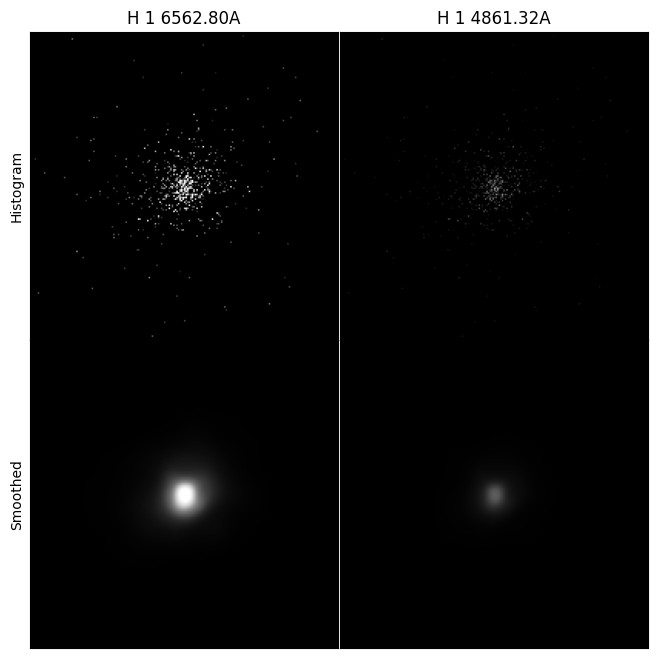
We use H-\(\alpha\) and H-\(\beta\) here: two of the most commonly used emission lines in the literature (star formation rate indicators, the Balmer decrement for dust attenuation, BPT diagrams, etc.), and bright enough in this galaxy to show clear structure.
[2]:
# Get the stellar pacman model - the same model used for photometric imaging,
# just queried for lines instead of (or as well as) spectra
model = BimodalPacmanEmission(
    grid=grid,
    tau_v_ism=1.0,
    tau_v_birth=0.7,
    dust_curve_ism=PowerLaw(slope=-1.3),
    dust_curve_birth=PowerLaw(slope=-0.7),
    fesc=0.1,
    fesc_ly_alpha=0.9,
    label="total",
    per_particle=True,
)

# H-alpha and H-beta
line_ids = ["H 1 6562.80A", "H 1 4861.32A"]

# Generate the per-particle lines
lines = gal.get_lines(line_ids, model)
print(lines)
+---------------------------------------------------------------------------------------------+
|                                       LINECOLLECTION                                        |
+--------------------+------------------------------------------------------------------------+
| Attribute          | Value                                                                  |
+--------------------+------------------------------------------------------------------------+
| nlines             | 2                                                                      |
+--------------------+------------------------------------------------------------------------+
| line2index         | mappingproxy({np.str_('H 1 6562.80A'): 0, np.str_('H 1 4861.32A'): 1}) |
+--------------------+------------------------------------------------------------------------+
| ndim               | 1                                                                      |
+--------------------+------------------------------------------------------------------------+
| nlam               | 2                                                                      |
+--------------------+------------------------------------------------------------------------+
| shape              | (2,)                                                                   |
+--------------------+------------------------------------------------------------------------+
| _available_ratios  | [BalmerDecrement, ]                                                    |
+--------------------+------------------------------------------------------------------------+
| available_ratios   | [BalmerDecrement, ]                                                    |
+--------------------+------------------------------------------------------------------------+
| elements           | [H, H]                                                                 |
+--------------------+------------------------------------------------------------------------+
| line_ids           | ['H 1 6562.80A' 'H 1 4861.32A']                                        |
+--------------------+------------------------------------------------------------------------+
| lam                | [6562.8  4861.32] Å                                                    |
+--------------------+------------------------------------------------------------------------+
| luminosity         | [44014.26000375 10641.05374572] Lsun                                   |
+--------------------+------------------------------------------------------------------------+
| continuum          | [1.34519436e+28 4.46667130e+27] erg/(Hz*s)                             |
+--------------------+------------------------------------------------------------------------+
| cont               | [1.34519436e+28 4.46667130e+27] erg/(Hz*s)                             |
+--------------------+------------------------------------------------------------------------+
| continuum_llam     | [244663.36294748 148060.02387896] Lsun/Å                               |
+--------------------+------------------------------------------------------------------------+
| energy             | [1.88919658 2.55042238] eV                                             |
+--------------------+------------------------------------------------------------------------+
| equivalent_width   | [0.17989722 0.07186986] Å                                              |
+--------------------+------------------------------------------------------------------------+
| lum                | [44014.26000375 10641.05374572] Lsun                                   |
+--------------------+------------------------------------------------------------------------+
| nu                 | [4.56805720e+14 6.16689414e+14] Hz                                     |
+--------------------+------------------------------------------------------------------------+
| vacuum_wavelengths | [6564.61289406 4862.6779924 ] Å                                        |
+--------------------+------------------------------------------------------------------------+
Mapping
The last step before we can make any line maps is to define a LineImager with the resolution and line ids attached, plus the FOV, or width, of the maps. A LineImager is configured with line_ids instead of filters — everything else about the instrument works identically to a PhotometricImager.
[3]:
# Define the width and resolution of the map
width = 30 * kpc
resolution = width / 200

# Create a line imaging instrument
instrument = LineImager(
    label="DemoLineImager", resolution=resolution, line_ids=line_ids
)

print(f"Map width is {width:.2f} with {resolution:.2f} resolution")
Map width is 30.00 kpc with 0.15 kpc resolution
Now we have everything we need to make line maps. The main public interface is the high-level galaxy API: get_line_maps_luminosity for luminosity maps and get_line_maps_flux for flux maps, exactly mirroring get_images_luminosity/get_images_flux for photometric images. Both take the map properties defined above, the line_ids we want maps for, and the emission model label the lines were generated with (“total” in this case), and return a single ImageCollection containing
one line map (Image) per requested line id.
[4]:
# Get the SPH kernel
kernel_data = Kernel().get_kernel()

# Get the histogram line maps
hist_maps = gal.get_line_maps_luminosity(
    "total",
    line_ids=line_ids,
    instrument=instrument,
    fov=width,
    img_type="hist",
    kernel=kernel_data,
    kernel_threshold=1,
    cosmo=cosmo,
)

# Get the smoothed line maps
smooth_maps = gal.get_line_maps_luminosity(
    "total",
    line_ids=line_ids,
    instrument=instrument,
    fov=width,
    img_type="smoothed",
    kernel=kernel_data,
    kernel_threshold=1,
    cosmo=cosmo,
)
Maps generated using these getter methods are both returned and attached to the Galaxy and components depending on where the lines were calculated. In the example above, the “total” lines were calculated on the Stars component, so the maps are attached to gal.stars under gal.stars.line_maps_lnu.
[5]:
# Lets set up a simple normalisation across all maps
vmax = 0
for img in hist_maps.values():
    up = np.percentile(img.arr, 99.9)
    if up > vmax:
        vmax = up
hist_norm = cm.Normalize(vmin=0, vmax=vmax)
vmax = 0
for img in smooth_maps.values():
    up = np.percentile(img.arr, 99.9)
    if up > vmax:
        vmax = up
smooth_norm = cm.Normalize(vmin=0, vmax=vmax)


# Set up plot
fig = plt.figure(figsize=(4 * len(line_ids), 4 * 2))
gs = gridspec.GridSpec(2, len(line_ids), hspace=0.0, wspace=0.0)

# Create top row
axes = []
for i in range(len(line_ids)):
    axes.append(fig.add_subplot(gs[0, i]))

# Loop over maps plotting them
for ax, line_id in zip(axes, line_ids):
    ax.imshow(hist_maps[line_id].arr, norm=hist_norm, cmap="Greys_r")
    ax.set_title(line_id)
    ax.tick_params(
        axis="both",
        which="both",
        left=False,
        right=False,
        labelleft=False,
        labelright=False,
        bottom=False,
        top=False,
        labelbottom=False,
        labeltop=False,
    )

# Set y axis label on left most plot
axes[0].set_ylabel("Histogram")

# Create bottom row
axes = []
for i in range(len(line_ids)):
    axes.append(fig.add_subplot(gs[1, i]))

# Loop over maps plotting them
for ax, line_id in zip(axes, line_ids):
    ax.imshow(smooth_maps[line_id].arr, norm=smooth_norm, cmap="Greys_r")
    ax.tick_params(
        axis="both",
        which="both",
        left=False,
        right=False,
        labelleft=False,
        labelright=False,
        bottom=False,
        top=False,
        labelbottom=False,
        labeltop=False,
    )

# Set y axis label on left most plot
axes[0].set_ylabel("Smoothed")

# Plot the map
plt.show()
plt.close(fig)
Flux maps
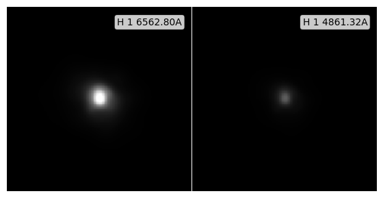
Just as with photometric images, we can also make flux line maps using get_line_maps_flux, once the observed lines have been calculated with get_observed_lines.
[6]:
gal.get_observed_lines(cosmo)

flux_maps = gal.get_line_maps_flux(
    "total",
    line_ids=line_ids,
    instrument=instrument,
    fov=width,
    img_type="smoothed",
    kernel=kernel_data,
    kernel_threshold=1,
    cosmo=cosmo,
)

fig, ax = flux_maps.plot_images(show=True)
plt.close(fig)
Blended lines
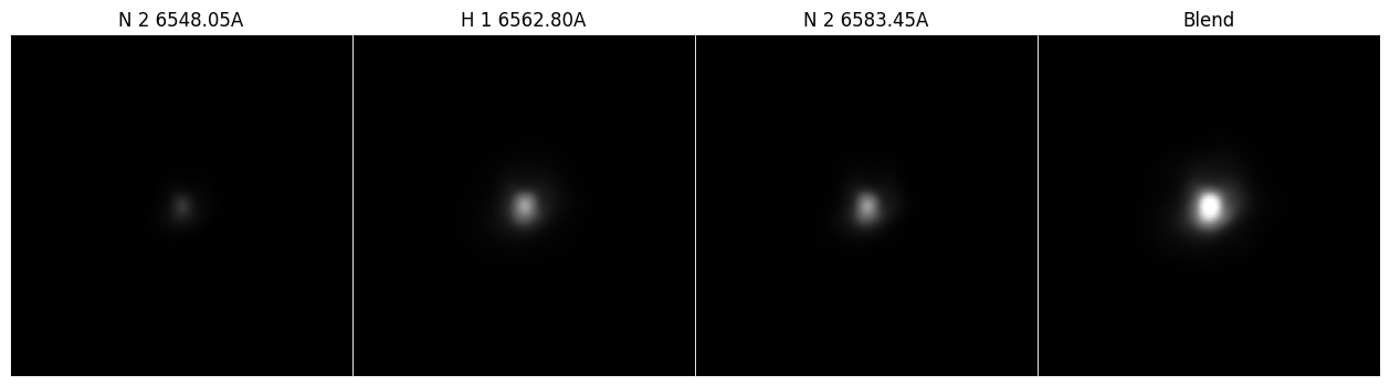
Lines that are close in wavelength are often unresolved by an instrument and observed as a single blended line. A classic example is H-\(\alpha\), which sits between the [NII] 6548, 6583 Å doublet: a narrow band filter targeting H-\(\alpha\) captures all three lines.
A blended line can be mapped directly by passing a nested list of line ids (or equivalently a comma separated string, e.g. "N 2 6548.05A, H 1 6562.80A, N 2 6583.45A") to both the LineImager and the getter. The resulting map is the sum of the component line maps, keyed by the component ids joined with ", ". Any per-line instrument inputs (PSFs, depths, noise maps) must use that same key.
The component lines must be available on the galaxy, so we first generate the [NII] lines alongside H-\(\alpha\). Here we map the blend alongside each of its components.
[7]:
# H-alpha and the [NII] doublet either side of it
halpha_nii = ["N 2 6548.05A", "H 1 6562.80A", "N 2 6583.45A"]

# Generate the component lines
gal.get_lines(halpha_nii, model)

# A nested list defines a blended line, here we map the blend and each of
# its components
blend_line_ids = [halpha_nii, *halpha_nii]
blend_instrument = LineImager(
    label="BlendLineImager", resolution=resolution, line_ids=blend_line_ids
)

blend_maps = gal.get_line_maps_luminosity(
    "total",
    line_ids=blend_line_ids,
    instrument=blend_instrument,
    fov=width,
    img_type="smoothed",
    kernel=kernel_data,
    kernel_threshold=1,
    cosmo=cosmo,
)

# The blended map is keyed by the joined line ids
blend_id = ", ".join(halpha_nii)
print(list(blend_maps.keys()))

# And is the sum of the component maps
component_sum = sum(blend_maps[line_id].arr for line_id in halpha_nii)
print(np.allclose(blend_maps[blend_id].arr, component_sum))
['N 2 6548.05A, H 1 6562.80A, N 2 6583.45A', 'N 2 6548.05A', 'H 1 6562.80A', 'N 2 6583.45A']
True
[8]:
# Plot each component alongside the blend on a common normalisation
panels = [*halpha_nii, blend_id]
titles = [*halpha_nii, "Blend"]
norm = cm.Normalize(vmin=0, vmax=np.percentile(blend_maps[blend_id].arr, 99.9))

fig = plt.figure(figsize=(4 * len(panels), 4))
gs = gridspec.GridSpec(1, len(panels), wspace=0.0)
for i, (line_id, title) in enumerate(zip(panels, titles)):
    ax = fig.add_subplot(gs[0, i])
    ax.imshow(blend_maps[line_id].arr, norm=norm, cmap="Greys_r")
    ax.set_title(title)
    ax.set_xticks([])
    ax.set_yticks([])

plt.show()
plt.close(fig)
That’s the core line mapping workflow. For PSF application, noise, RGB maps, and angular vs Cartesian imaging — all of which work identically for line maps, just keyed by line id instead of filter code — see the particle imaging notebook.