Parametric Star Formation Histories
Parametric SFH Models
All parametric SFH models in Synthesizer inherit from the Common SFH base class. This ensures a consistent interface and shared functionality across different SFH implementations. SFHs are typically dimensionless, representing the relative star formation rate over time. The overall normalization is handled by the stellar mass of the Stars component the SFH is associated with.
[1]:
%load_ext autoreload
%autoreload 2

from unyt import yr

from synthesizer.parametric import SFH
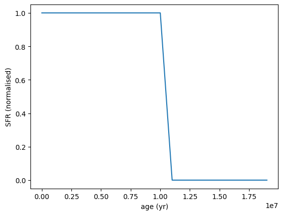
Constant SFH
The simplest SFH model is the constant star formation history, which assumes a uniform star formation rate over time. This is controlled by minimum and maximum age parameters.
[2]:
sfh = SFH.Constant(min_age=0 * yr, max_age=1e7 * yr)

sfh.plot_sfh(t_range=(0, 2e7))
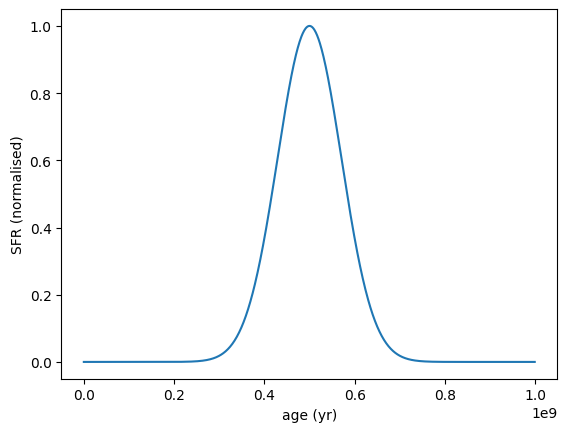
Gaussian SFH
A Gaussian SFH models star formation as a Gaussian function over time, characterized by a mean age and standard deviation. This allows for modeling scenarios where star formation peaks at a certain epoch and tapers off.
[3]:
sfh = SFH.Gaussian(peak_age=5e8 * yr, sigma=1e8 * yr)

sfh.plot_sfh(t_range=(0, 1e9))
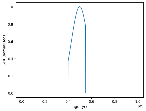
Note that all SFHs have a separate min_age and max_age parameter that define the valid age range for the SFH. Outside this range the SFH will return zero, which is useful for truncating SFHs.
Here’s an example of a Gaussian SFH with specified minimum and maximum ages:
[4]:
sfh = SFH.Gaussian(
    peak_age=5e8 * yr, sigma=1e8 * yr, min_age=4e8 * yr, max_age=5.5e8 * yr
)
sfh.plot_sfh(t_range=(0, 1e9))
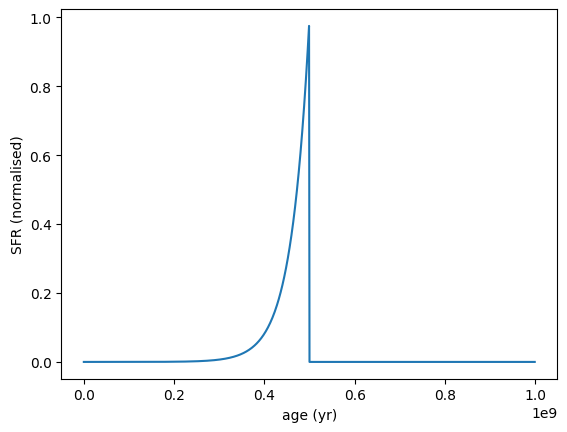
Exponential SFH
An Exponential SFH models star formation as an exponential function over time, characterized by a timescale parameter (tau). This allows for modelling scenarios where star formation either rises or declines exponentially.
It is parameterized by:
tau: The e-folding timescale of the SFH. A positive value indicates an exponentially declining SFH, while a negative value indicates an exponentially rising SFH.min_age: The minimum age for which the SFH is defined.max_age: The maximum age for which the SFH is defined.
Postive tau (declining SFH) example:
[5]:
sfh = SFH.Exponential(tau=4e7 * yr, max_age=5e8 * yr)
sfh.plot_sfh(t_range=(0, 1e9))
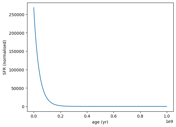
Negative tau (rising SFH) example:
[6]:
sfh = SFH.Exponential(tau=-4e7 * yr, max_age=5e8 * yr)
sfh.plot_sfh(t_range=(0, 1e9))
Truncated Exponential SFH
This is an alias for an ExponentialSFH, as all SFH classes have min_age and max_age parameters that define the valid age range for the SFH. Outside this range the SFH will return zero.
Declining Exponential SFH
This is also an alias for an ExponentialSFH with a positive tau value, as all SFH classes have min_age and max_age parameters that define the valid age range for the SFH. Outside this range the SFH will return zero.
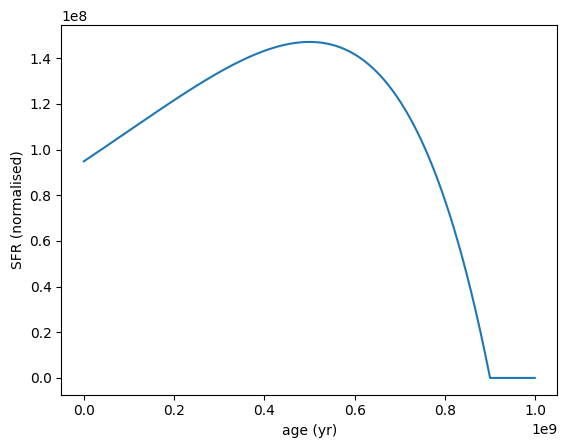
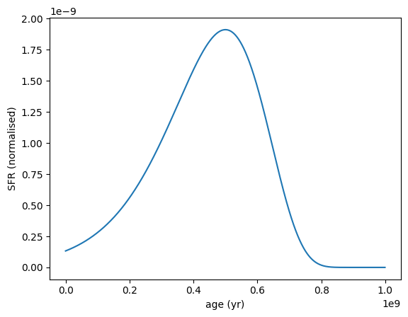
Delayed Exponential SFH
A Delayed Exponential SFH models star formation as a function that rises linearly to a peak and then declines exponentially. This is useful for scenarios where star formation ramps up before declining.
It is parameterized by:
tau: The e-folding timescale of the SFH.min_age: The minimum age for which the SFH is defined.max_age: The maximum age for which the SFH is defined.
[7]:
sfh = SFH.DelayedExponential(tau=4e8 * yr, max_age=9e8 * yr)

sfh.plot_sfh(t_range=(0, 1e9))
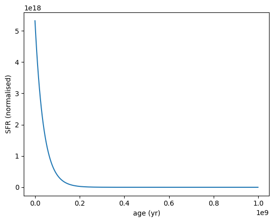
Negative tau will produce a rising SFH.
[8]:
sfh = SFH.DelayedExponential(tau=-4e7 * yr, max_age=9e8 * yr)
sfh.plot_sfh(t_range=(0, 1e9))
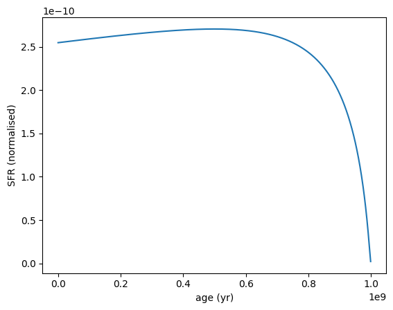
Lognormal SFH
A Lognormal SFH models star formation as a lognormal function over time, characterized by a mean and standard deviation in logarithmic space. This allows for modeling scenarios where star formation has a skewed distribution over time.
It is parameterized by:
tau: A dimensionless parameter that controls the width of the lognormal distribution.peak_age: The age at which the SFH peaks.min_age: The minimum age for which the SFH is defined.max_age: The maximum age for which the SFH is defined.
Higher tau values result in broader SFHs, while lower tau values produce narrower SFHs. Note that max_age should be greater than peak_age to ensure the SFH is defined over the desired range.
max_age is a required parameter which will scale the SFH.
[9]:
sfh = SFH.LogNormal(tau=0.3, peak_age=5e8 * yr, max_age=1e9 * yr)

sfh.plot_sfh(t_range=(0, 1e9))
Broader tau example:
[10]:
sfh = SFH.LogNormal(tau=2, peak_age=5e8 * yr, max_age=1e9 * yr)

sfh.plot_sfh(t_range=(0, 1e9))
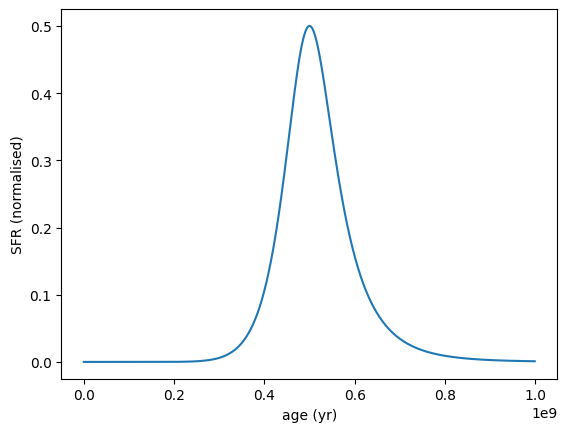
Double Power Law SFH
A Double Power Law SFH models star formation as a piecewise function with two power-law segments, allowing for more flexibility in capturing the evolution of star formation rates over time. It is characterized by a break age, which separates the two power-law regimes.
It is parameterized by:
peak_age: The age at which the SFH transitions between the two power-law segments.alpha: The power-law index for the rising segment of the SFH.beta: The power-law index for the declining segment of the SFH.min_age: The minimum age for which the SFH is defined.max_age: The maximum age for which the SFH is defined.
Note that alpha should be positive to ensure a rising SFH before the peak, and beta should be negative to ensure a declining SFH after the peak. max_age should be greater than peak_age to ensure the SFH is defined over the desired range.
[11]:
sfh = SFH.DoublePowerLaw(
    peak_age=5e8 * yr, alpha=10, beta=-10, max_age=1e9 * yr
)

sfh.plot_sfh(t_range=(0, 1e9))
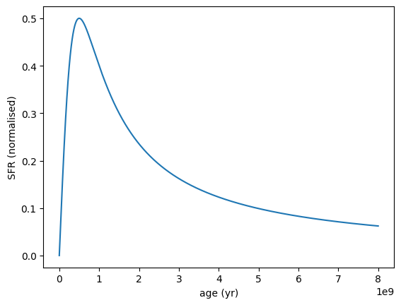
Modelling a recently quenched galaxy with a sharp peak:
[12]:
sfh = SFH.DoublePowerLaw(peak_age=5e8 * yr, alpha=1, beta=-1, max_age=8e9 * yr)

sfh.plot_sfh(t_range=(0, 8e9))
Drawing SFHs from priors
All parametric SFH models have an init_from_prior class method that allows users to generate random SFH realizations based on specified prior ranges. For parametric models this is currently limited to uniform priors on each parameter.
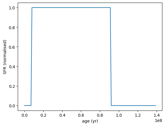
This is set by passing in tuples defining parameter ranges for each model parameter. For example, to generate a Constant SFH with a minimum age between 0 and 10 Myr, and a maximum age between 10 Myr and 100 Myr, you would do the following:
[13]:
sfh = SFH.Constant.init_from_prior(
    min_age=(0, 1e7) * yr, max_age=(1e7, 1e8) * yr
)

sfh.plot_sfh(t_range=(0, 1.4e8))
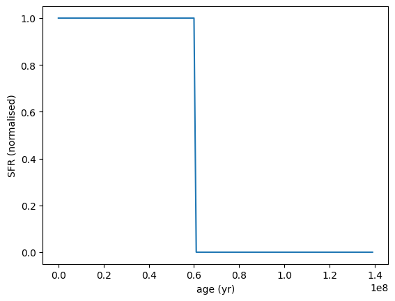
Note that for parameters that are not specified as ranges, you can provide fixed values directly.
[14]:
sfh = SFH.Constant.init_from_prior(min_age=0 * yr, max_age=(1e7, 1e8) * yr)

sfh.plot_sfh(t_range=(0, 1.4e8))
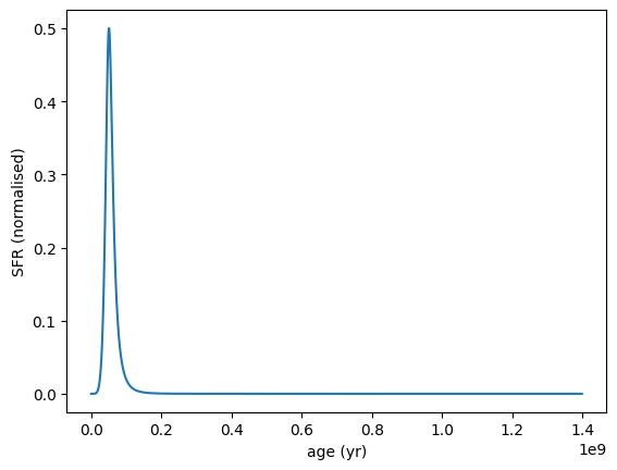
Here’s a more complex example using the Double Power Law SFH:
[15]:
sfh = SFH.DoublePowerLaw.init_from_prior(
    peak_age=(1e7, 1e9) * yr,
    alpha=(0.1, 20),
    beta=(-20, -0.1),
    min_age=0 * yr,
    max_age=2e9 * yr,
)

sfh.plot_sfh(t_range=(0, 1.4e9))
‘Non-parametric’ SFH Models
The next section will cover non-parametric SFH models, which allow for more complex and flexible representations of star formation histories without relying on predefined functional forms.
These star formation history models are generally powerful because they can capture a wide range of SFH shapes, including bursts, quenching events, and other complex behaviors that may not be well-represented by simple parametric forms. They are typically controlled by one or more hyperparameters that influence the overall shape and smoothness of the SFH. These hyperparameters are not set if the SFH is set directly by the user, but these SFHs all have a method to draw samples from the prior defined by the hyperparameters.
This method is called init_from_prior and can be used to generate random SFH realizations based on the specified hyperparameters. This is particularly useful for exploring the range of possible SFHs that are consistent with the chosen model and its priors.
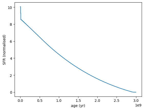
Dense Basis SFH
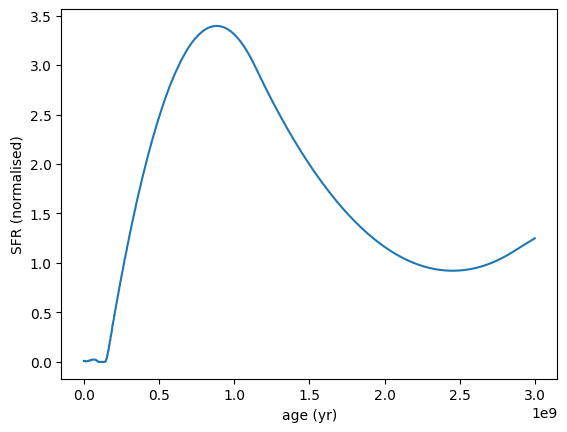
The Dense Basis SFH (Iyer et al. 2017, 2019) is a Gaussian Process based SFH model that uses combinations of Gaussian functions to represent complex star formation histories. This approach allows for a flexible and data-driven representation of SFHs, capturing a wide range of possible star formation scenarios. See here for more details.
The Dense Basis SFH is modelled by a overall stellar mass normalization, a recent SFR, and a set of N lookback times at which the galaxy has formed N equal mass fractions.
It is parameterized by:
db_tuple: A tuple defining the Dense Basis parameters.redshift: The redshift at which the SFH is evaluated. This is required to calculate the age of the universe and properly scale the SFH.
The db_tuple includes the following parameters in the specified order:
total mass formed (in log10 solar masses). Note that this is not important for the SFH shape, as the overall normalization is handled by the
Starscomponent.recent SFR (in log10 solar masses per year).
Number of lookback times (N).
N lookback times at which the galaxy has formed N equal mass fractions. These are scaled between 0 and 1, where 0 corresponds to the present day and 1 corresponds to the age of the universe at the specified redshift.
Please cite Iyer et al. (2017, 2019) when using this SFH model in your work.
[16]:
logmass = 10
logsfr = 1
nparams = 1
frac_mass_formed = 0.9
redshift = 1


db_tuple = (logmass, logsfr, nparams, frac_mass_formed)
sfh = SFH.DenseBasis(db_tuple, redshift=redshift)

sfh.plot_sfh(t_range=(0, 3e9))
sklearn not available. The `gp_sklearn` interpolator will fail if chosen.
Starting dense_basis. Failed to load FSPS, only GP-SFH module will be available.
running without emcee
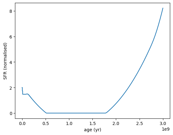
Here’s a recently quenched SFH, where we’ve specified 3 different lookback times for the equal mass fractions.
[17]:
logmass = 10
logsfr = -2
nparams = 3
frac_mass_formed = (0.25, 0.5, 0.8)
redshift = 1


db_tuple = (logmass, logsfr, nparams, *frac_mass_formed)
sfh = SFH.DenseBasis(db_tuple, redshift=redshift)

sfh.plot_sfh(t_range=(0, 3e9))
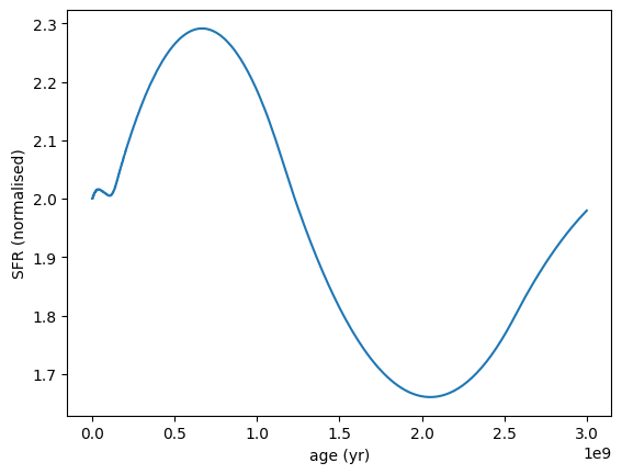
Now for all non-parametric SFH models we can use the init_from_prior method to generate random SFH realizations based on specified hyperparameters. This allows us to explore the range of possible SFHs that are consistent with the chosen model and its priors.
For the DenseBasis SFH model, we specify a tx_alpha hyperparameter that controls the distribution of the lookback times. Higher values of tx_alpha will result in lookback times that are more evenly distributed, while lower values have more randomness, leading to more bursty SFHs.
tx_alpha = 5.0 example:
[18]:
sfh = SFH.DenseBasis.init_from_prior(
    N_tx=3, log_mass=10, log_sfr=0.3, redshift=1, tx_alpha=5.0
)

sfh.plot_sfh(t_range=(0, 3e9))
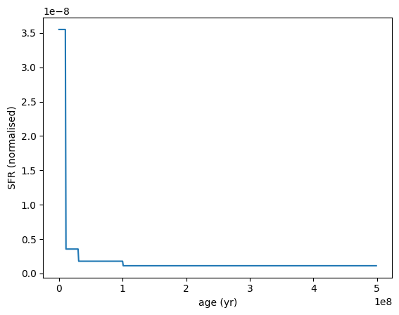
tx_alpha = 1.0 example:
[19]:
sfh = SFH.DenseBasis.init_from_prior(
    N_tx=3, log_mass=10, log_sfr=0.3, redshift=1, tx_alpha=1.0
)

sfh.plot_sfh(t_range=(0, 3e9))
Continuity SFH
This SFH was introduced by Leja et al. (2019) and is a time-binned non-parametric SFH model that enforces continuity between adjacent time bins. This approach helps to produce smoother and more physically realistic star formation histories by penalizing abrupt changes in the star formation rate.
The model is controlled by the SFR ratio between adjacent time bins, which are controlled by a Dirichlet prior. This encourages the SFH to vary smoothly over time, avoiding unphysical jumps in the star formation rate.
The concentration parameter of the Dirichlet prior determines how strongly continuity is enforced. A higher concentration value results in a smoother SFH, while a lower value allows for more variability between time bins.
This SFH is parameterized by:
logsfr_ratios: The logarithm of the SFR ratios between adjacent time bins. This is an array of length N-1, where N is the number of time bins.agebins: The edges of the time bins in which the SFH is defined. This is a 2D array with shape (N, 2), where each row defines the start and end of a time bin.min_age: The minimum age for which the SFH is defined.max_age: The maximum age for which the SFH is defined.
Please cite Leja et al. (2019) when using this SFH model in your work.
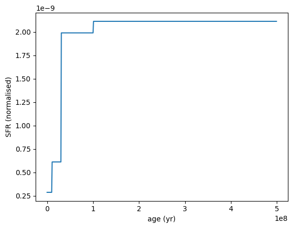
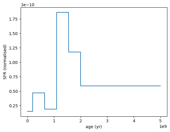
Here’s a recently rising SFH, with bins from 0-10 Myr, 10-30 Myr, 30-100 Myr and 100-500 Myr. Note that as we have specified the logsfr_ratios directly, the continuity prior is not applied here.
[20]:
logsfr_ratios = [1, 0.3, 0.2]
agebins = [[0, 1e7], [1e7, 3e7], [3e7, 1e8], [1e8, 5e8]] * yr
sfh = SFH.Continuity(logsfr_ratios=logsfr_ratios, agebins=agebins)

sfh.plot_sfh(t_range=(0, 5e8))
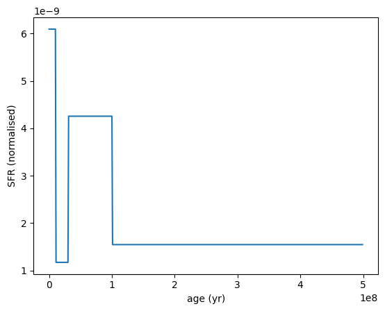
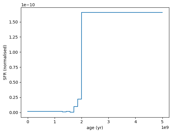
Here’s an example where we draw a random SFH from the continuity prior, using the same age bins as above.
[21]:
sfh = SFH.Continuity.init_from_prior(agebins=agebins)
sfh.plot_sfh(t_range=(0, 5e8))
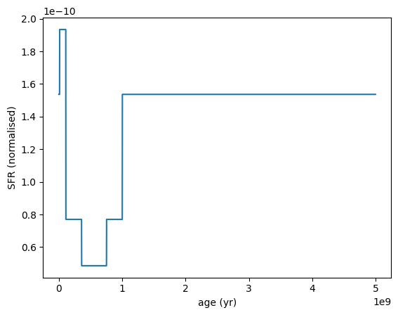
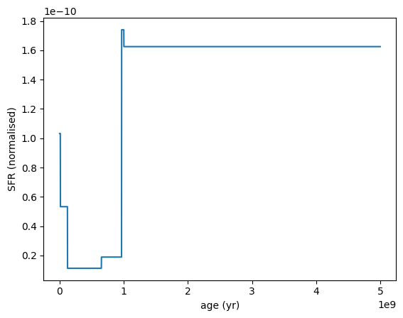
Often called the ‘bursty continuity’ prior, if we change the concentration parameter of the Dirichlet prior from 2 to 0.3, we allow for more bursty SFHs with larger variations between adjacent time bins. Here’s an example of such a bursty SFH drawn from the prior.
[22]:
sfh = SFH.Continuity.init_from_prior(agebins=agebins, scale=0.3)
sfh.plot_sfh(t_range=(0, 5e8))
ContinuityFlex SFH
The ContinuityFlex SFH is an extension of the Continuity SFH model, which introduces specific agebins for young and old stellar populations, with intermediate agebins distributed logarithmically in between.
The model is parameterized by:
logsfr_ratios_young: The logarithm of the SFR ratios between adjacent time bins for the young stellar population.logsfr_ratios_old: The logarithm of the SFR ratios between adjacent time bins for the old stellar population.logsfr_ratios: The logarithm of the SFR ratios between adjacent time bins for the intermediate agebins.fixed_young_bin: A two component array defining the edges of the young stellar population age bin.fixed_old_bin: A two component array defining the edges of the old stellar population agemin_age: The minimum age for which the SFH is defined.max_age: The maximum age for which the SFH is defined.
Here’s an example of a Continuity SFH with specified SFR ratios and age bins:
[23]:
sfh = SFH.ContinuityFlex(
    logsfr_ratio_young=-0.1,
    logsfr_ratio_old=0.3,
    logsfr_ratios=[0.4, 0.2, -0.2],
    fixed_young_bin=[0, 1e7] * yr,
    fixed_old_bin=[1e9, 7e9] * yr,
)

sfh.plot_sfh(t_range=(0, 5e9))
We can also draw random SFHs from the prior using the init_from_prior method. In this example, we specify 3 intermediate agebins between the fixed young and old bins.
[24]:
sfh = SFH.ContinuityFlex.init_from_prior(
    N_flex_bins=3, fixed_young_bin=[0, 1e7] * yr, fixed_old_bin=[1e9, 7e9] * yr
)


sfh.plot_sfh(t_range=(0, 5e9))
ContinuityPSB SFH
Introduced by Suess et al. 2021, the ContinuityPSB SFH is a variation of the Continuity SFH model that is specifically designed to capture the star formation histories of post-starburst galaxies. This model incorporates a burst of star formation followed by a rapid decline, which is characteristic of post-starburst galaxies.
It uses a combination of fixed-width and flexible-boundary time bins to model the star formation history (SFH). A smoothness prior, based on a Student’s t-distribution, is applied to the logarithmic ratios of SFRs in adjacent time bins.
The time bins are structured from youngest to oldest as follows:
A single “youngest” bin of variable width
tlast.A set of
nflexbins spanning the time fromtlasttotflex.A set of
nfixedbins spanning the time fromtflextomax_age.
[25]:
sfh = SFH.ContinuityPSB(
    logsfr_ratio_young=-0.5,
    logsfr_ratio_old=[0.3, -0.2, 0.1],
    logsfr_ratios=[0.4, -1.0, 0.2],
    tlast=0.2e9 * yr,
    tflex=2e9 * yr,
    nflex=4,
    nfixed=3,
    max_age=13e9 * yr,
)

sfh.plot_sfh(t_range=(0, 5e9))
We can also draw random SFHs from the prior using the init_from_prior method.
[26]:
sfh = SFH.ContinuityPSB.init_from_prior()

sfh.plot_sfh(t_range=(0, 5e9))
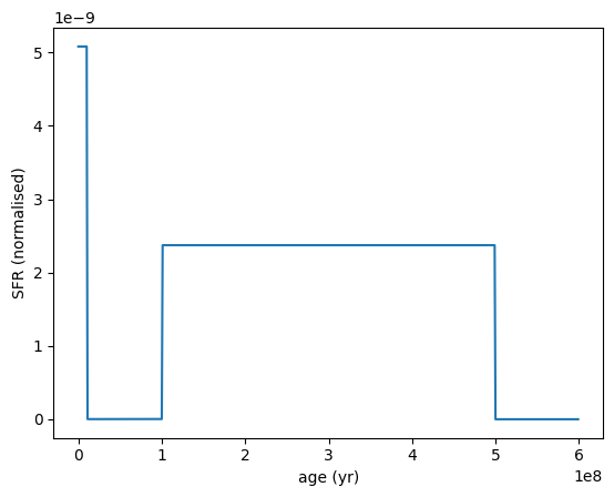
Dirichlet SFH
The Dirichlet SFH is a time-binned non-parametric SFH model that uses a Dirichlet prior to define the star formation rates in each time bin. The Dirichlet prior uses independent Beta-distributed variables that are transformed to SFR fractions which sum to unity.
[27]:
sfh = SFH.Dirichlet(
    z_fraction=[0.2, 0.5, 0.8],
    agebins=[[0, 1e7], [1e7, 3e7], [3e7, 1e8], [1e8, 5e8]] * yr,
)

sfh.plot_sfh(t_range=(0, 6e8))
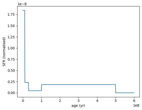
Here we draw a random SFH from the Dirichlet prior with specified age bins and Beta distribution parameters. Note that we can specify the loc and scale parameters of the Beta distribution to control the shape of the prior.
[28]:
sfh = SFH.Dirichlet.init_from_prior(
    agebins=[[0, 1e7], [1e7, 3e7], [3e7, 1e8], [1e8, 5e8]] * yr,
    loc=1.0,
    scale=0.3,
)

sfh.plot_sfh(t_range=(0, 6e8))
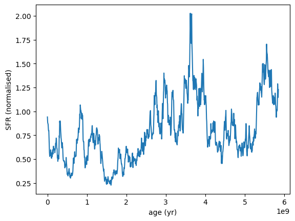
Stochastic SFH
The Stochastic SFH (Iyer et al. 2024, arXiv:2208.05938) draws a star formation history as a Gaussian Process realisation in log-SFR space. Fluctuations about a mean (base) SFH are drawn from a covariance kernel, following the Power Spectral Density formalism in which different physical processes imprint variability on different timescales.
The variability model is encapsulated in a separate Kernels object, so new models can be added without changing the SFH class. The simplest kernel is the DampedRandomWalk (a single-timescale regulator), whose log-SFR auto-covariance is \(C(\Delta t) = \sigma^2\, e^{-|\Delta t| / \tau}\):
sigmasets the amplitude of the variability (in dex of log10 SFR),tausets the correlation timescale (largetaugives smooth SFHs, smalltaugives bursty SFHs).
Because the SFH is a stochastic realisation, it depends on the observation redshift (which sets the age of the universe, and hence the time baseline) and a random_seed.
[29]:
from unyt import Gyr

from synthesizer.parametric import Kernels

kernel = Kernels.DampedRandomWalk(sigma=0.3, tau=1 * Gyr)
sfh = SFH.Stochastic(redshift=1, kernel=kernel, random_seed=42)

sfh.plot_sfh(t_range=(0, sfh.t_univ))
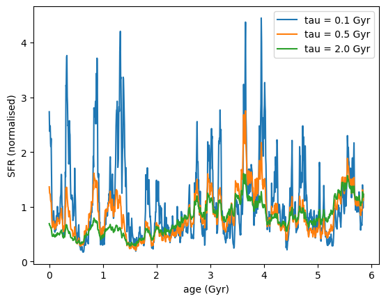
The correlation timescale tau controls how bursty the SFH is. A long tau produces smooth, slowly varying histories, while a short tau produces rapid, bursty variability (all drawn here with the same seed):
[30]:
import matplotlib.pyplot as plt

fig, ax = plt.subplots()
for tau in [0.1, 0.5, 2.0]:
    kernel = Kernels.DampedRandomWalk(sigma=0.3, tau=tau * Gyr)
    sfh = SFH.Stochastic(redshift=1, kernel=kernel, random_seed=42)
    t, s = sfh.calculate_sfh(t_range=(0, sfh.t_univ))
    ax.plot(t / 1e9, s, label=f"tau = {tau} Gyr")

ax.set_xlabel("age (Gyr)")
ax.set_ylabel("SFR (normalised)")
ax.legend()
plt.show()
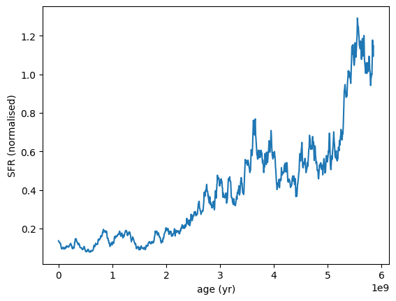
By default the fluctuations sit on top of a flat (constant) mean SFH, but base_sfh is pluggable: you can pass a callable f(t_cosmic_yr) -> SFR (or an array on the internal grid) to impose a mean trend, e.g. an exponentially declining mean SFH:
[31]:
import numpy as np

kernel = Kernels.DampedRandomWalk(sigma=0.2, tau=1 * Gyr)
sfh = SFH.Stochastic(
    redshift=1,
    kernel=kernel,
    base_sfh=lambda t: np.exp(-t / 3e9),
    random_seed=42,
)

sfh.plot_sfh(t_range=(0, sfh.t_univ))
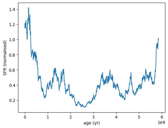
As with the other models, the kernel parameters can be drawn from (uniform) priors via the kernel’s own init_from_prior method:
[32]:
kernel = Kernels.DampedRandomWalk.init_from_prior(
    sigma=[0.1, 0.5], tau=[0.5, 3.0] * Gyr
)
sfh = SFH.Stochastic(redshift=1, kernel=kernel, random_seed=7)

sfh.plot_sfh(t_range=(0, sfh.t_univ))
Combined SFH
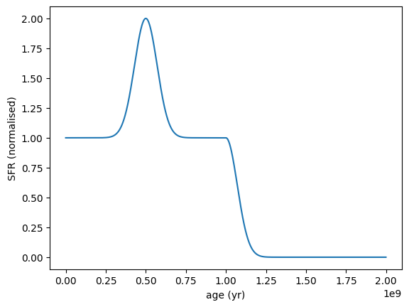
The CombinedSFH class allows for the combination of multiple SFH models into a single composite SFH. This is useful for modeling complex star formation histories that may involve multiple distinct phases or components. As SFHs are normalized, the CombinedSFH accepts a weight for each component SFH to control their relative contributions to the overall SFH.
Here’s an example of a Constant SFH combined with two Gaussian SFHs to create a more complex star formation history.
[33]:
sfh1 = SFH.Constant(min_age=0 * yr, max_age=1e9 * yr)
sfh2 = SFH.Gaussian(
    peak_age=5e8 * yr, sigma=1e8 * yr, min_age=0 * yr, max_age=3e9 * yr
)
sfh3 = SFH.Gaussian(
    peak_age=1e9 * yr, sigma=1e8 * yr, min_age=1.0001e9 * yr, max_age=3e9 * yr
)

combined_sfh = SFH.CombinedSFH(
    sfhs=[sfh1, sfh2, sfh3],
    weights=[1.0, 1.0, 1.0],
)

combined_sfh.plot_sfh(t_range=(0, 2e9))