The Grid Object

Here we show how to instantiate a Grid object and use it to explore a grid file.

The Grid object needs a file to load, these are HDF5 files that are available through the synthesizer-download command line tool (for more details see the introduction to grids. By default, once downloaded these files are stored in the GRID_DIR directory. The default location of this directory is platform dependent, but the location can be found by import it and printing it.

from synthesizer import GRID_DIR

print(GRID_DIR)

/home/runner/.local/share/Synthesizer/grids

This directory can be overriden by setting the SYNTHESIZER_GRID_DIR environment variable.

Assuming the grid file is in the default location, all we need to do is pass the name of the grid we want to load to the Grid constructor. Note that the name of the grid can include the extension or not. If the extension is not included, it is assumed to be "hdf5".

Here we will load the test grid (a simplified BPASS 2.2.1 grid).

from synthesizer import Grid

grid = Grid("test_grid.hdf5")

If we are loading a grid from a different location we can just pass that path to the grid_dir argument.

grid = Grid(
    "test_grid.hdf5", grid_dir="../../../tests/test_grid", ignore_lines=True
)

Printing a summary of the Grid

We can have a look at what the loaded grid contains by simply printing the grid.

print(grid)

+-----------------------------------------------------------------------------------+
|                                       GRID                                        |
+-----------------------------+-----------------------------------------------------+
| Attribute                   | Value                                               |
+-----------------------------+-----------------------------------------------------+
| grid_dir                    | '../../../tests/test_grid'                          |
+-----------------------------+-----------------------------------------------------+
| grid_name                   | 'test_grid'                                         |
+-----------------------------+-----------------------------------------------------+
| grid_ext                    | 'hdf5'                                              |
+-----------------------------+-----------------------------------------------------+
| grid_filename               | '../../../tests/test_grid/test_grid.hdf5'           |
+-----------------------------+-----------------------------------------------------+
| reprocessed                 | True                                                |
+-----------------------------+-----------------------------------------------------+
| naxes                       | 2                                                   |
+-----------------------------+-----------------------------------------------------+
| date_created                | '2025-03-05'                                        |
+-----------------------------+-----------------------------------------------------+
| synthesizer_grids_version   | '0.1.dev613+ga9a6aa9'                               |
+-----------------------------+-----------------------------------------------------+
| synthesizer_version         | '0.8.5b1.dev124+ge16216b5'                          |
+-----------------------------+-----------------------------------------------------+
| has_lines                   | False                                               |
+-----------------------------+-----------------------------------------------------+
| has_spectra                 | True                                                |
+-----------------------------+-----------------------------------------------------+
| lines_available             | False                                               |
+-----------------------------+-----------------------------------------------------+
| ndim                        | 3                                                   |
+-----------------------------+-----------------------------------------------------+
| new_line_format             | False                                               |
+-----------------------------+-----------------------------------------------------+
| nlam                        | 9244                                                |
+-----------------------------+-----------------------------------------------------+
| nlines                      | 0                                                   |
+-----------------------------+-----------------------------------------------------+
| shape                       | (51, 13, 9244)                                      |
+-----------------------------+-----------------------------------------------------+
| available_spectra_emissions | [incident, linecont, nebular, transmitted,          |
|                             |  nebular_continuum, ]                               |
+-----------------------------+-----------------------------------------------------+
| available_emissions         | [linecont, nebular_continuum, nebular, transmitted, |
|                             |  incident, ]                                        |
+-----------------------------+-----------------------------------------------------+
| axes                        | [ages, metallicities]                               |
+-----------------------------+-----------------------------------------------------+
| available_spectra           | [incident, linecont, nebular, transmitted,          |
|                             |  nebular_continuum, ]                               |
+-----------------------------+-----------------------------------------------------+
| lam (9244,)                 | 1.30e-04 Å -> 2.99e+11 Å (Mean: 9.73e+09 Å)         |
+-----------------------------+-----------------------------------------------------+
| incident_axes               | ['ages' 'metallicities']                            |
+-----------------------------+-----------------------------------------------------+
| spec_names (4,)             | [incident, transmitted, nebular, ...]               |
+-----------------------------+-----------------------------------------------------+
| spectra                     | incident: ndarray                                   |
|                             | linecont: ndarray                                   |
|                             | nebular: ndarray                                    |
|                             | transmitted: ndarray                                |
|                             | nebular_continuum: ndarray                          |
+-----------------------------+-----------------------------------------------------+
| _axes_values                | ages: ndarray                                       |
|                             | metallicities: ndarray                              |
+-----------------------------+-----------------------------------------------------+
| log10_specific_ionising_lum | HI: ndarray                                         |
|                             | HeII: ndarray                                       |
+-----------------------------+-----------------------------------------------------+
| axes_values                 | ages: ndarray                                       |
|                             | metallicities: ndarray                              |
+-----------------------------+-----------------------------------------------------+

In this instance, its a stellar grid with the incident spectrum defined by the axes_values, ages and metallicities. The grid also contains some useful quantites like the photon rate (log10_specific_ionising_luminosity) available for fully ionising hydrogen and helium.

Since this grid is a cloudy processed grid, there are additional spectra or line data that are available to extract or manipulate. These include (but not limited to)

• spectra

  • nebular: is the nebular continuum (including line emission) predicted by the photoionisation model

  • linecont: this is the line contribution to the spectrum

  • transmitted: this is the incident spectra that is transmitted through the gas in the photoionisation modelling; it has zero flux at shorter wavelength of the lyman-limit

  • wavelength: the wavelength covered

• lines

  • id: line id, this is the same as used in cloudy (see Linelist generation)

  • luminosity: the luminosity of the line

  • nebular_continuum: the underlying nebular continuum at the line

  • transmitted: this is the transmitted luminosity at the line

  • wavelength: the wavelength of the line

A similar structure is also followed for AGN grids, where the axes could either be described by mass (black hole mass), acretion_rate_eddington (the accretion rate normalised to the eddington limit for the mass), cosine_inclination (cosine value describing the inclination of the AGN), or the temperature (blackbody temperature of the big bump component), alpha-ox (X-ray to UV ratio) , alpha-uv (low-energy slope of the big bump component), alpha-x (slope of the X-ray component).

Limiting the Grid

A Grid can be limited in various ways to reduce memory usage and focus on specific wavelength regions or parameter ranges. This can be done either during instantiation or after the grid is loaded using dedicated reduction methods.

Limiting during instantiation

Passing a wavelength array

If you only care about a grid of specific wavelength values, you can pass this array and the Grid will automatically be interpolated onto the new wavelength array at instantiation using SpectRes.

# Define a new set of wavelengths
new_lams = np.logspace(2, 5, 1000) * angstrom

# Create a new grid
grid = Grid(
    "test_grid",
    # ignore_lines=True,
    new_lam=new_lams,
)
print(grid.shape)

(51, 13, 1000)

Passing wavelength limits

If you don’t want to modify the underlying grid resolution, but only care about a specific wavelength range, you can instead pass limits to truncate the grid at instantiation.

# Create a new grid
grid = Grid("test_grid", lam_lims=(10**3 * angstrom, 10**4 * angstrom))
print(grid.shape)

(51, 13, 692)

/tmp/ipykernel_6525/3897584189.py:2: RuntimeWarning:
The following lines are outside the wavelength range of the grid: [np.str_('H 1
1.00494m'), np.str_('S 2 1.02867m'), np.str_('S 2 1.03205m'), np.str_('S 2
1.03364m'), np.str_('He 1 1.08291m'), np.str_('He 1 1.08303m'), np.str_('H 1
1.09381m'), np.str_('O 1 1.12863m'), np.str_('O 1 1.12864m'), np.str_('O 1
1.12869m'), np.str_('O 1 1.12870m'), np.str_('O 1 1.12873m'), np.str_('Ni 2
1.19102m'), np.str_('Fe 2 1.25668m'), np.str_('Fe 2 1.27877m'), np.str_('H 1
1.28181m'), np.str_('Fe 2 1.29427m'), np.str_('Fe 2 1.32055m'), np.str_('Fe 2
1.32777m'), np.str_('Fe 2 1.37181m'), np.str_('Fe 2 1.53348m'), np.str_('Fe 2
1.59948m'), np.str_('Fe 2 1.64355m'), np.str_('Fe 2 1.66377m'), np.str_('Fe 2
1.67688m'), np.str_('Fe 2 1.71113m'), np.str_('Fe 2 1.74494m'), np.str_('Fe 2
1.79711m'), np.str_('Fe 2 1.80002m'), np.str_('Fe 2 1.80940m'), np.str_('H 1
1.87510m'), np.str_('Fe 2 1.89541m'), np.str_('Ni 2 1.93877m'), np.str_('Fe 2
1.95361m'), np.str_('Si 6 1.96247m'), np.str_('H 1 2.16553m'), np.str_('Si 7
2.48071m')]
  grid = Grid("test_grid", lam_lims=(10**3 * angstrom, 10**4 * angstrom))

Ignoring spectra or lines

It is also possible to ignore either spectra or lines. This can be useful if, for example, you have a large multi-dimensional grid and only want to consider lines since these are much smaller in memory.

# Create a new grid without spectra
grid = Grid("test_grid", ignore_spectra=True)

print(grid.available_spectra)

# Create a new grid without lines
grid = Grid("test_grid", ignore_lines=True)

[]

Grid reduction methods

Beyond limiting during instantiation, grids can also be modified after loading using dedicated reduction methods. These methods return a new Grid object by default, leaving the original grid unchanged. For in-place modification, you can add inplace=True to any reduction method and this will instead modify the existing grid.

Wavelength range reduction

You can reduce a grid to a specific rest-frame wavelength range.

# Load a fresh grid
grid = Grid("test_grid")
print(
    f"Original wavelength range: {grid.lam.min():.0f} - {grid.lam.max():.0f}"
)
print(f"Original grid shape: {grid.shape}")

# Reduce to a specific rest-frame wavelength range (UV-optical)
# Returns a new grid by default, leaving the original unchanged
reduced_grid = grid.reduce_rest_frame_range(1000 * angstrom, 8000 * angstrom)
print(
    f"Reduced wavelength range: {reduced_grid.lam.min():.0f} - "
    f"{reduced_grid.lam.max():.0f}"
)
print(f"Reduced grid shape: {reduced_grid.shape}")

Original wavelength range: 0 Å - 299293000000 Å
Original grid shape: (51, 13, 9244)
Reduced wavelength range: 999 Å - 7995 Å
Reduced grid shape: (51, 13, 625)

/tmp/ipykernel_6525/3661447593.py:10: RuntimeWarning:
52 lines are outside the wavelength range of the grid and will be removed.
  reduced_grid = grid.reduce_rest_frame_range(1000 * angstrom, 8000 * angstrom)

Notice that the code warns you if any lines are now outside the wavelength range and have been removed.

You can also limit to an observer-frame wavelength range at a specific redshift.

# Load a fresh grid
grid = Grid("test_grid")

# Reduce to observed wavelength range at redshift z=1
redshift = 1.0
reduced_grid = grid.reduce_observed_range(
    2000 * angstrom, 8000 * angstrom, redshift
)
print(
    f"Rest-frame range after observed reduction: "
    f"{reduced_grid.lam.min():.0f} - {reduced_grid.lam.max():.0f}"
)
print(f"Grid shape: {reduced_grid.shape}")

Rest-frame range after observed reduction: 999 Å - 3997 Å
Grid shape: (51, 13, 417)

/tmp/ipykernel_6525/4284589168.py:6: RuntimeWarning:
126 lines are outside the wavelength range of the grid and will be removed.
  reduced_grid = grid.reduce_observed_range(

You can also reduce to a specific wavelength array (via interpolation using SpectRes).

# Load a fresh grid
grid = Grid("test_grid")

# Define a custom wavelength array (lower resolution)
custom_lam = np.logspace(2.5, 4.5, 500) * angstrom

# Reduce the grid to this wavelength array
reduced_grid = grid.reduce_rest_frame_lam(custom_lam)
print(f"New wavelength points: {len(reduced_grid.lam)}")
print(f"Grid shape: {reduced_grid.shape}")
print(f"Original grid unchanged: {len(grid.lam)} wavelength points")

New wavelength points: 500
Grid shape: (51, 13, 500)
Original grid unchanged: 9244 wavelength points

Which can also be done in the observer-frame at a specific redshift.

# Load a fresh grid
grid = Grid("test_grid")

# Define a custom observed wavelength array (lower resolution)
redshift = 1.0
custom_lam = np.logspace(2.5, 4.5, 500) * angstrom * (1 + redshift)

# Reduce the grid to this wavelength array at the specified redshift
reduced_grid = grid.reduce_observed_lam(custom_lam, redshift)
print(f"New wavelength points: {len(reduced_grid.lam)}")
print(f"Grid shape: {reduced_grid.shape}")

New wavelength points: 500
Grid shape: (51, 13, 500)

Filter-based reduction

You can reduce a grid to the non-zero transmission wavelength range of a set of filters. Again, this can be done in either the rest-frame or observer-frame at a specific redshift.

from synthesizer.instruments.filters import UVJ

# Load a fresh grid
grid = Grid("test_grid")

# Get UVJ filter collection
filters = UVJ()
print(f"Filter effective wavelengths: {[f.lam_eff for f in filters]}")

# Reduce grid to rest-frame filter range
reduced_grid = grid.reduce_rest_frame_filters(filters)
print(
    f"Grid reduced to filter range: {reduced_grid.lam.min():.0f} - "
    f"{reduced_grid.lam.max():.0f}"
)
print(f"Grid shape: {reduced_grid.shape}")

# You can also reduce to observer-frame filter ranges
# For in-place modification, use inplace=True
redshift = 2.0
grid.reduce_observed_filters(filters, redshift, inplace=True)
print(
    f"Grid reduced for z={redshift} observations (in-place): "
    f"{grid.lam.min():.0f} - {grid.lam.max():.0f}"
)

Filter effective wavelengths: [unyt_quantity(3650, 'Å'), unyt_quantity(5510, 'Å'), unyt_quantity(12200, 'Å')]
Grid reduced to filter range: 3317 Å - 13269 Å
Grid shape: (51, 13, 159)
Grid reduced for z=2.0 observations (in-place): 1108 Å - 4417 Å

/tmp/ipykernel_6525/314517307.py:11: RuntimeWarning:
90 lines are outside the wavelength range of the grid and will be removed.
  reduced_grid = grid.reduce_rest_frame_filters(filters)
/tmp/ipykernel_6525/314517307.py:21: RuntimeWarning:
115 lines are outside the wavelength range of the grid and will be removed.
  grid.reduce_observed_filters(filters, redshift, inplace=True)

Parameter axis reduction

Instead of limiting the wavelength range, you might instead be interested in limiting the parameter space of the grid. This can be done using the reduce_axis method.

# Load a fresh grid
grid = Grid("test_grid")
print(
    f"Original (log10) age range: {grid.log10ages.min():.1f} - "
    f"{grid.log10ages.max():.1f}"
)
print(
    f"Original metallicity range: {grid.metallicities.min():.3f} - "
    f"{grid.metallicities.max():.3f}"
)
print(f"Original grid shape: {grid.shape}")

# Reduce to young stellar populations only (log age < 7.5)
age_reduced_grid = grid.reduce_axis(6, 7.5, "log10ages")
print(
    f"Reduced age range: {age_reduced_grid.log10ages.min():.1f} - "
    f"{age_reduced_grid.log10ages.max():.1f}"
)
print(f"Grid shape after age reduction: {age_reduced_grid.shape}")

# Further reduce to low metallicity (Z < 0.02)
final_grid = age_reduced_grid.reduce_axis(
    age_reduced_grid.metallicities.min(), 0.02, "metallicities"
)
print(
    f"Reduced metallicity range: {final_grid.metallicities.min():.3f} - "
    f"{final_grid.metallicities.max():.3f}"
)
print(f"Final grid shape: {final_grid.shape}")

Original (log10) age range: 6.0 - 11.0
Original metallicity range: 0.000 dimensionless - 0.040 dimensionless
Original grid shape: (51, 13, 9244)
Reduced age range: 0.8 - 0.9
Grid shape after age reduction: (16, 13, 9244)
Reduced metallicity range: 0.000 dimensionless - 0.020 dimensionless
Final grid shape: (16, 11, 9244)

You can chain these calls together in a single line if you want to.

# Load a fresh grid
grid = Grid("test_grid")

reduced_grid = grid.reduce_axis(6, 7.5, "log10ages").reduce_axis(
    grid.metallicities.min(), 0.01, "metallicities"
)
print("Original grid shape:", grid.shape)
print("Reduced grid shape:", reduced_grid.shape)

Original grid shape: (51, 13, 9244)
Reduced grid shape: (16, 9, 9244)

Grid collapse methods

Beyond reduction, you can also collapse entire parameter dimensions using various methods:

Marginalization

Collapse a dimension by marginalizing (e.g., averaging) over it:

# Load a fresh grid
grid = Grid("test_grid")
print(f"Original axes: {grid.axes}")
print(f"Original shape: {grid.shape}")

# Collapse over metallicity by averaging
collapsed_grid = grid.collapse(
    "metallicities", method="marginalize", marginalize_function=np.mean
)
print(f"Axes after collapse: {collapsed_grid.axes}")
print(f"Shape after collapse: {collapsed_grid.shape}")
print(f"Original grid unchanged: {grid.axes}")

Original axes: ['ages', 'metallicities']
Original shape: (51, 13, 9244)
Axes after collapse: ['ages']
Shape after collapse: (51, 9244)
Original grid unchanged: ['ages', 'metallicities']

Interpolation to specific values

Collapse a dimension by interpolating to a specific parameter value:

# Load a fresh grid
grid = Grid("test_grid")

# Collapse to a specific age (log10(age) = 6.5)
target_age = 6.5
collapsed_grid = grid.collapse(
    "log10ages", method="interpolate", value=target_age
)
print(f"Collapsed to log10(age) = {target_age}")
print(f"Remaining axes: {collapsed_grid.axes}")
print(f"Shape after collapse: {collapsed_grid.shape}")
print(f"Original grid unchanged: {grid.axes}")

Collapsed to log10(age) = 6.5
Remaining axes: ['metallicities']
Shape after collapse: (13, 9244)
Original grid unchanged: ['ages', 'metallicities']

Nearest value extraction

Collapse by extracting the nearest grid point:

# Load a fresh grid
grid = Grid("test_grid")

# Collapse to nearest metallicity value
target_Z = 0.015
collapsed_grid = grid.collapse(
    "metallicities", method="nearest", value=target_Z
)
print(f"Collapsed to nearest Z = {target_Z}")
print(f"Remaining axes: {collapsed_grid.axes}")
print(f"Shape after collapse: {collapsed_grid.shape}")
print(f"Original grid unchanged: {grid.axes}")

Collapsed to nearest Z = 0.015
Remaining axes: ['ages']
Shape after collapse: (51, 9244)
Original grid unchanged: ['ages', 'metallicities']

Combining methods for efficient workflows

These methods can be combined for efficient analysis workflows:

# Example: Focus on young, metal-poor stars in the optical
# Method 1: Chain operations (returns new grids each time)
grid = Grid("test_grid")
print(f"Starting grid shape: {grid.shape}")

# Chain the operations - each returns a new grid
final_grid = (
    grid.reduce_rest_frame_range(
        3000 * angstrom, 7000 * angstrom
    )  # 1. Optical wavelengths
    .reduce_axis(
        grid.log10ages.min(), 7.0, "log10ages"
    )  # 2. Young populations
    .collapse("metallicities", method="nearest", value=0.02)
)  # 3. Solar metallicity

print(f"Final grid shape: {final_grid.shape}")
print(f"Original grid unchanged: {grid.shape}")

# Method 2: In-place operations (modifies the same grid)
grid2 = Grid("test_grid")
print("\nAlternative approach - modifying in-place:")
print(f"Starting grid shape: {grid2.shape}")

# Modify the grid in-place
grid2.reduce_rest_frame_range(3000 * angstrom, 7000 * angstrom, inplace=True)
print(f"After wavelength reduction: {grid2.shape}")

grid2.reduce_axis(grid2.log10ages.min(), 7.0, "log10ages", inplace=True)
print(f"After age reduction: {grid2.shape}")

grid2.collapse("metallicities", method="nearest", value=0.02, inplace=True)
print(f"After metallicity collapse: {grid2.shape}")

Starting grid shape: (51, 13, 9244)
Final grid shape: (11, 255)
Original grid unchanged: (51, 13, 9244)

Alternative approach - modifying in-place:
Starting grid shape: (51, 13, 9244)
After wavelength reduction: (51, 13, 255)
After age reduction: (11, 13, 255)
After metallicity collapse: (11, 255)

/tmp/ipykernel_6525/4222753654.py:8: RuntimeWarning:
131 lines are outside the wavelength range of the grid and will be removed.
  grid.reduce_rest_frame_range(
/tmp/ipykernel_6525/4222753654.py:26: RuntimeWarning:
131 lines are outside the wavelength range of the grid and will be removed.
  grid2.reduce_rest_frame_range(3000 * angstrom, 7000 * angstrom, inplace=True)

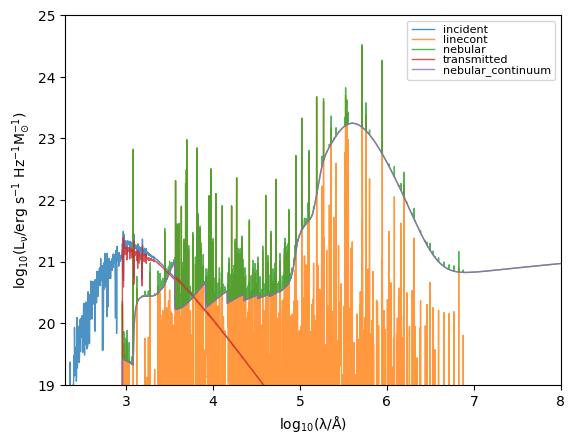
Plot a single grid point

We can plot the spectra at the location of a single point in our grid. First, we choose some age and metallicity.

# Return to the unmodified grid
grid = Grid("test_grid")

log10age = 6.0  # log10(age/yr)
Z = 0.01  # metallicity

We then get the index location of that grid point for this age and metallicity

grid_point = grid.get_grid_point(log10ages=log10age, metallicity=Z)

We can then loop over the available spectra (contained in grid.spec_names) and plot

for spectra_type in grid.available_spectra:
    # Get `Sed` object
    sed = grid.get_sed_at_grid_point(grid_point, spectra_type=spectra_type)

    # Mask zero valued elements
    mask = sed.lnu > 0
    plt.plot(
        np.log10(sed.lam[mask]),
        np.log10(sed.lnu[mask]),
        lw=1,
        alpha=0.8,
        label=spectra_type,
    )

plt.legend(fontsize=8, labelspacing=0.0)
plt.xlim(2.3, 8)
plt.ylim(19, 25)
plt.xlabel(r"$\rm log_{10}(\lambda/\AA)$")
plt.ylabel(r"$\rm log_{10}(L_{\nu}/erg\ s^{-1}\ Hz^{-1} M_{\odot}^{-1})$")

Text(0, 0.5, '$\\rm log_{10}(L_{\\nu}/erg\\ s^{-1}\\ Hz^{-1} M_{\\odot}^{-1})$')

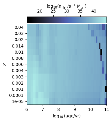
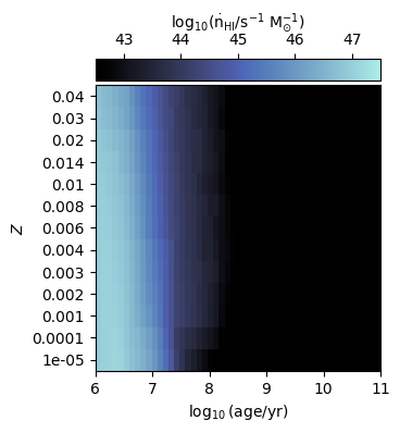
Plot ionising luminosities

We can also plot properties over the entire age and metallicity grid, such as the ionising luminosity.

In the examples below we plot ionising luminosities for HI and HeII

fig, ax = grid.plot_specific_ionising_lum(ion="HI")

fig, ax = grid.plot_specific_ionising_lum(ion="HeII")