Intergalactic Medium Absorption

Neutral hydrogen in the intergalactic medium (IGM) attenuates the light from distant galaxies, even after reionisation. Synthesizer provides three analytic forms for this IGM absorption: Madau96, Inoue14, and Asada25.

The Madau96 model is based on Madau et al. (1996), and assumes a power-law relationship between the absorption and the redshift.

The Inoue14 model is based on Inoue et al. (2014), and includes the effects of the Lyman-\(\alpha\) forest and Lyman–limit systems.

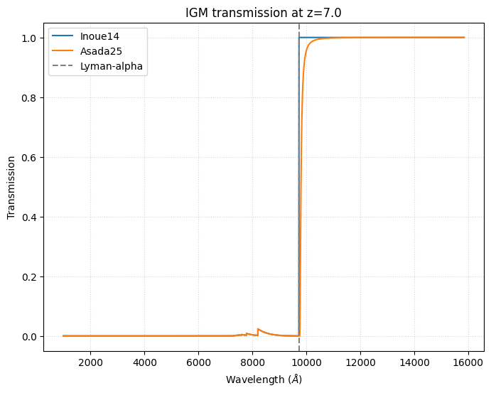
The Asada25 model is based on Asada et al. 2025, and extends the Inoue14 model by including additional Circumgalactic Medium (CGM) absorption at high redshifts (z>6). This model uses the Inoue+14 IGM prescription with an additional Lyα damping wing component calibrated from high-redshift observations.

Plotting the transmission curves

To simply visualize the transmission curves, we can simply instantiate the IGM class and call the plot_transmission method, passing our desired redshift and wavelength array (in Angstroms).

import numpy as np
from unyt import angstrom

from synthesizer.emission_models.attenuation import Asada25, Inoue14, Madau96

madau = Madau96()
inoue = Inoue14()
asada = Asada25()

# Define redshift and wavelength range
redshift = 5.0
lams = np.logspace(3, 4, 10000) * angstrom

fig, ax = madau.plot_transmission(redshift, lams)
_, _ = inoue.plot_transmission(redshift, lams, fig=fig, ax=ax, show=False)
_, _ = asada.plot_transmission(redshift, lams, fig=fig, ax=ax, show=False)
ax.axvline(
    x=1216 * (1 + redshift), label="Lyman-break", ls="dashed", color="grey"
)
ax.legend()
ax.grid(ls="dotted", alpha=0.5)

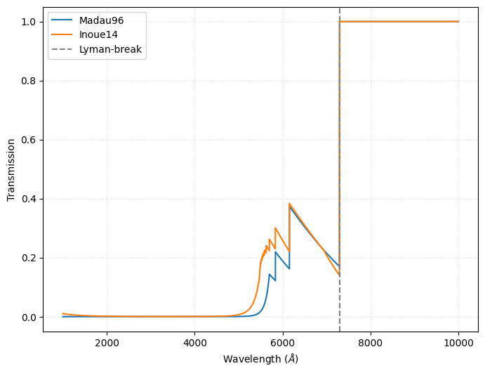
Notice that we have passed the fig and ax to get all models on the same plot. This can be done with all of Synthesizer’s plotting methods.

The Asada25 model becomes particularly important at high redshifts (z>6). Let’s compare the models at z=7:

# Compare at high redshift where CGM effects become important
redshift_high = 7.0
lams_high = np.logspace(3, 4.2, 10000) * angstrom

fig, ax = inoue.plot_transmission(redshift_high, lams_high)
_, _ = asada.plot_transmission(
    redshift_high, lams_high, fig=fig, ax=ax, show=False
)
ax.axvline(
    x=1216 * (1 + redshift_high),
    label="Lyman-alpha",
    ls="dashed",
    color="grey",
)
ax.legend()
ax.grid(ls="dotted", alpha=0.5)
ax.set_title(f"IGM transmission at z={redshift_high}")

Text(0.5, 1.0, 'IGM transmission at z=7.0')

Using the IGM models for attenuation

In reality most of the time you will not be working with the IGM models directly, but rather using them to attenuate your spectra. This is done automatically when a Sed (docs here) is converted to fluxes, all you need to do is pass the desired (uninstatiated) IGM model to get_fnu.

Below we will use the Madau96 model to attenuate a spectrum extracted from a Grid (docs here).

from astropy.cosmology import Planck18 as cosmo

from synthesizer.grid import Grid

grid_name = "test_grid"
grid = Grid(grid_name)

log10age = 6.0  # log10(age/yr)
metallicity = 0.01
grid_point = grid.get_grid_point(log10ages=log10age, metallicity=metallicity)
sed = grid.get_sed_at_grid_point(grid_point, spectra_type="transmitted")
sed.lnu *= 1e8  # multiply initial stellar mass

# Compute the flux in the presence of IGM attenuation
sed.get_fnu(cosmo=cosmo, z=redshift, igm=Madau96)

unyt_array([0., 0., 0., ..., 0., 0., 0.], shape=(9244,), units='nJy')

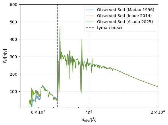
Below we plot the spectra produced when assuming each of the models for IGM attenuation:

# Plot the intrinsic and observed SED
fig, ax = sed.plot_observed_spectra(
    figsize=(6, 6), show=False, label="Observed SED (Madau 1996)"
)
sed.get_fnu(cosmo=cosmo, z=redshift, igm=Inoue14)
_, _ = sed.plot_observed_spectra(
    fig=fig,
    ax=ax,
    show=False,
    label="Observed SED (Inoue 2014)",
    xlimits=(5000, 20000),
    ylimits=(10, 600),
)
sed.get_fnu(cosmo=cosmo, z=redshift, igm=Asada25)
_, _ = sed.plot_observed_spectra(
    fig=fig,
    ax=ax,
    show=False,
    label="Observed SED (Asada 2025)",
    xlimits=(5000, 20000),
    ylimits=(10, 600),
)
ax.axvline(
    x=1216 * (1 + redshift), label="Lyman-break", ls="dashed", color="grey"
)
ax.legend(framealpha=0.3)
ax.grid(ls="dotted", alpha=0.5)
ax.set_yscale("linear")

Customizing the Asada25 model

The Asada25 model allows customization of the sigmoid parameters that control the CGM HI column density evolution. You can also disable the CGM component to recover the Inoue+14 behavior:

# Create Asada25 models with different settings
asada_default = Asada25()  # Default parameters
asada_no_cgm = Asada25(add_cgm=False)  # Without CGM (equivalent to Inoue14)
asada_custom = Asada25(
    sigmoid_params=(4.0, 2.0, 19.0)
)  # Custom sigmoid parameters

# Compare at z=8 where CGM effects are strongest
z_test = 8.0
lams_test = np.logspace(3, 4, 10000) * angstrom

fig, ax = asada_default.plot_transmission(z_test, lams_test)
_, _ = asada_no_cgm.plot_transmission(
    z_test, lams_test, fig=fig, ax=ax, show=False
)
_, _ = asada_custom.plot_transmission(
    z_test, lams_test, fig=fig, ax=ax, show=False
)
ax.set_title(f"Asada25 model variations at z={z_test}")
ax.legend()
ax.grid(ls="dotted", alpha=0.5)