Pipeline Profiling
These benchmarks represent “real-world” usage patterns where multiple operations are performed in sequence using the Pipeline object. This tests how the full pipeline scales with problem size when performing all typical analysis tasks together.
Test Configuration
The Pipeline profiling uses the following configuration to represent realistic observational analysis workflows:
Emission Model |
|
Instrument |
JWST NIRCam Wide with 8 filters (F070W, F090W, F115W, F150W, F200W, F277W, F356W, F444W) |
Imaging |
60 kpc field of view at z=1.0 with angular resolution (0.031 arcsec/pixel) |
Operations Performed |
LOS optical depths, SFZH/SFH (star formation history), rest-frame spectra (Lnu), observer-frame spectra (Fnu), photometry luminosities, photometry fluxes, emission line luminosities, emission line fluxes, rest-frame images, observer-frame images |
Galaxies |
10 synthetic galaxies per run, each containing stars, gas, and black holes |
Particle Counts |
100, 500, 1000, 5000, 10000 |
Hardware |
AMD EPYC 7542 32-Core Processor, 8 threads used |
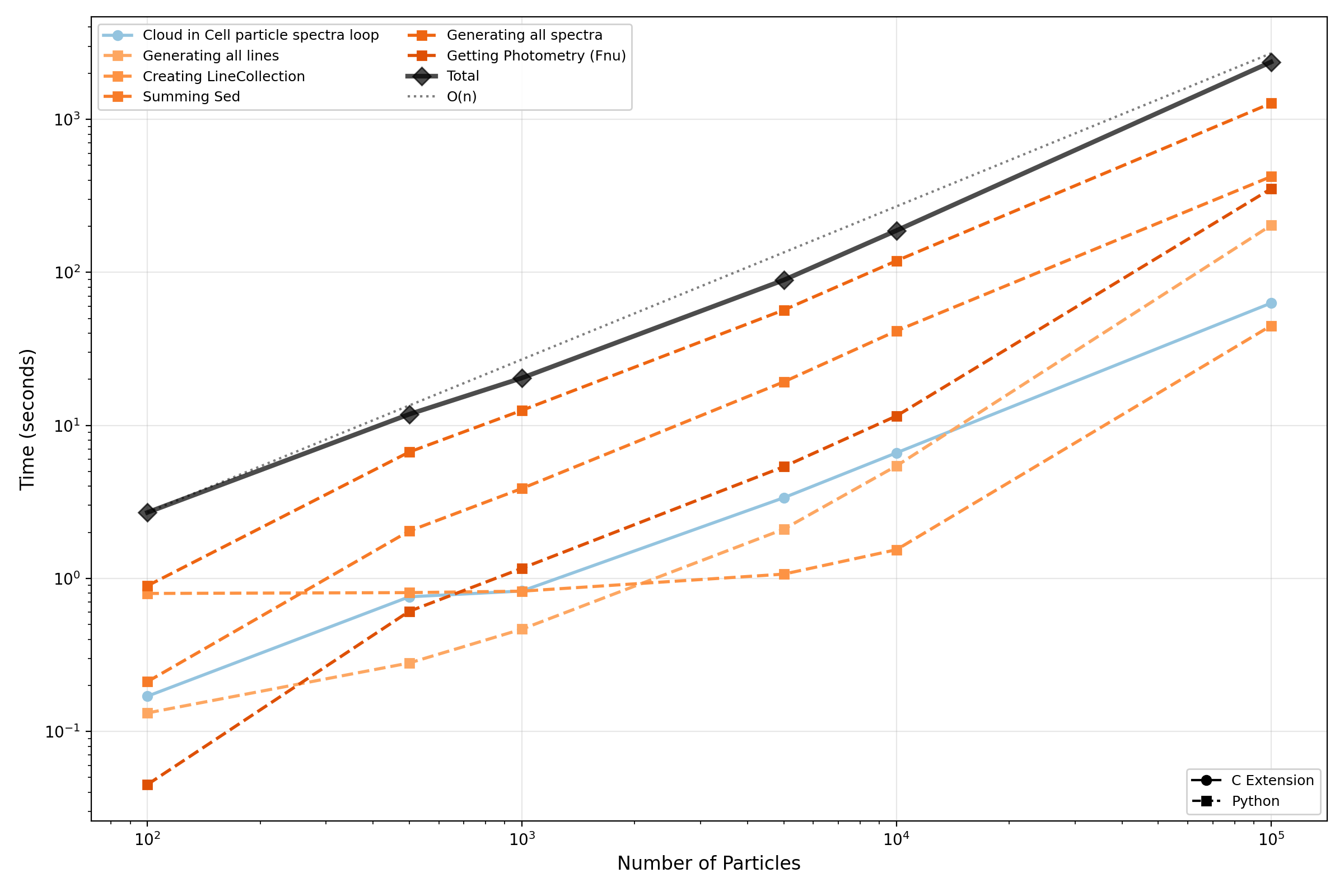
Timing Performance
The following plot shows how the Pipeline runtime scales with the number of stellar particles per galaxy. Only operations contributing ≥5% to the total runtime in at least one particle count are shown. The O(n) reference line is anchored at the first data point (100 particles).
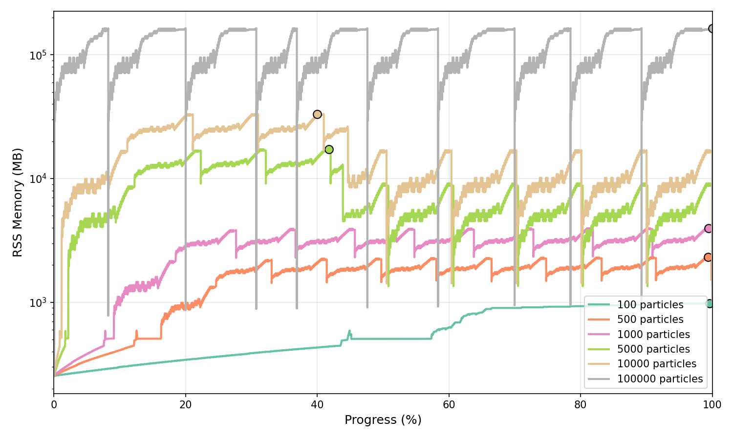
Memory Performance
The following plots show the memory usage (RSS sampling at high frequency) of the full Pipeline execution across different particle counts. Sampling frequencies range from 5 kHz for 100 particles down to 500 Hz for 10,000 particles to ensure adequate temporal resolution across all test cases.
Normalised Memory Profile
Memory usage normalised to execution progress (0-100%), shown in MB on a logarithmic scale. Peak memory is marked with circles.
Peak Memory Scaling
Peak memory vs particle count on log-log axes (shown in MB) with an O(n) reference line anchored at the first data point.
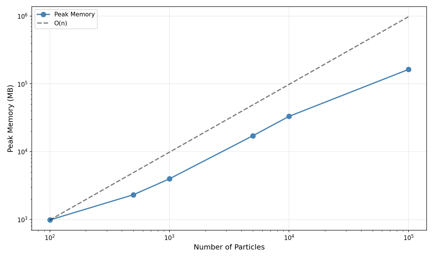
Memory Scaling Results:
Particle Count |
Peak Memory |
Scaling Factor |
|---|---|---|
100 |
882 MB |
1.0× (baseline) |
500 |
1,578 MB |
1.8× baseline |
1000 |
2,567 MB |
2.9× baseline |
5000 |
9,252 MB |
10.5× baseline |
10000 |
14,575 MB |
16.5× baseline |
Profiling Scripts
The Pipeline profiling can be reproduced using the scripts in the profiling/pipeline directory:
# Run timing profiling
python profile_timing.py --basename npart_1000 --nparticles 1000 \
    --ngalaxies 10 --include-observer-frame

# Run memory profiling (with custom sampling frequency)
python profile_memory.py --basename npart_1000 --nparticles 1000 \
    --ngalaxies 10 --sample-freq 2000 --include-observer-frame

# Analyse timing results
python analyse_timing.py --inputs npart_*/timing.csv \
    --labels "100" "500" "1000" --output-dir timing_analysis

# Analyse memory results
python analyse_memory.py --inputs npart_*/memory.csv \
    --labels "100" "500" "1000" --output-dir memory_analysis
See the profiling README for more details on running and customising the profiling suite.