Dust Attenuation Curves
We implement a whole suite of different attenuation curves in synthesizer, including the following:
PowerLaw: A power-law attenuation curve.Calzetti2000: The Calzetti (Calzetti et al. 2000) attenuation curve (with an optional UV bump from Noll et al. 2009).MWN18: A Milky Way attenuation curve, defined in Narayanan et al. 2018.GrainModels: A dust grain attenuation curve from the dust-extinction package. These models are based on dust grain size, composition, and shape distributions constrained by observations of extinction, abundances, emission, and polarization. Some of these models can be used to estimate extinction at wavelengths inaccessible to observation, e.g. X-ray wavelengths.ParametricLi08: A parametric and empirically derived attenuation curve implemented in Li et al. 2008, including parameters from Markov et al. 2023 and Markov et al. 2024.DraineLiGrainCurves: Extinction curves based on grain properties, using dust efficiency factors forgraphite,silicate,ionised PAH, andneutral PAHfrom Draine & Li. These curves are parameterised by the dust-to-gas ratio of each constituent grain component. Default grids are available; custom grids for different grain size bins can also be created (see the companiongrid-generationrepo)
These attenuation curves can be instantiated directly, or attached to an EmissionModel to be used in the generation of complex spectra from a galaxy or galaxy component.
Each model has unique arguments required at instantiation, but all have the same base methods, such as get_transmission (which requires an optical depth (tau_v, not for DraineLiGrainCurves though) and a wavelength array). Below, we show how to instantiate each of these models and plot their transmission and attenuation curves.
We first define a wavelength array up front:
[1]:
import numpy as np
from unyt import Angstrom

lams = np.logspace(3.1, 4, 10000) * Angstrom
PowerLaw
A PowerLaw only requires a slope to be defined. We can then use the in-built methods, e.g. get_transmission, to return the transmission over our wavelength array values.
[2]:
from synthesizer.emission_models.attenuation import PowerLaw

power_law = PowerLaw(-1.0)

pl_trans = power_law.get_transmission(0.33, lams)
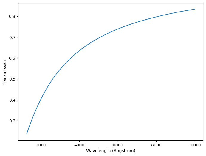
Below we plot the transmission and attenuation curves.
[3]:
power_law.plot_transmission(0.33, lams, show=True)
power_law.plot_attenuation(lams, show=True)
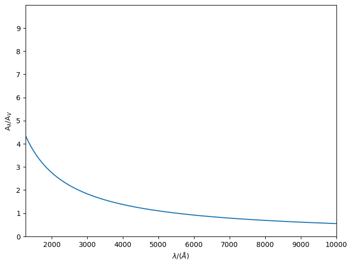
[3]:
(<Figure size 800x600 with 1 Axes>,
 <Axes: xlabel='$\\lambda/(\\AA)$', ylabel='A$_{\\lambda}/$A$_{V}$'>)
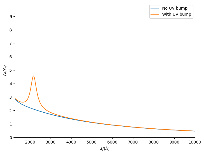
Calzetti2000
The Calzetti2000 model requires a slope (slope), central wavelength of the UV bump (cent_lam), amplitude of the UV bump (ampl), and the FWHM of the UV bump (gamma). These default to 0.0, 0.2175 microns, 0, and 0.035, respectively. We plot the transmission curve both with the defaults and a non-zero bump amplitude.
[4]:
from synthesizer.emission_models.attenuation import Calzetti2000

no_bump = Calzetti2000()
with_bump = Calzetti2000(ampl=10.0)

fig, ax = no_bump.plot_attenuation(lams, show=False, label="No UV bump")
_, _ = with_bump.plot_attenuation(
    lams, fig=fig, ax=ax, show=True, label="With UV bump"
)
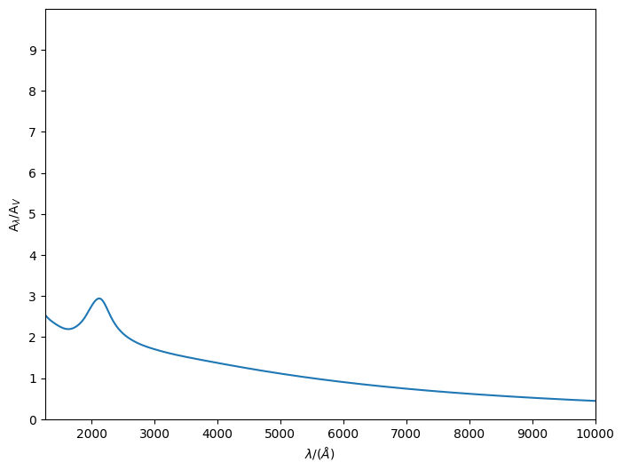
MWN18
The MWN18 model loads a data file included with synthesizer; as such, it requires no arguments.
[5]:
from synthesizer.emission_models.attenuation import MWN18

mwn18 = MWN18()

_, _ = mwn18.plot_attenuation(lams, show=True)
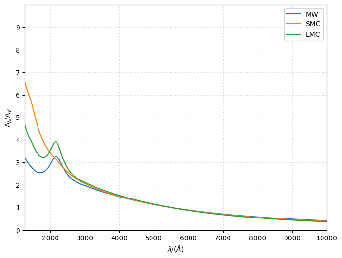
GrainModels
GrainModels requires the model (either 'DBP90', 'WD01', 'D03', 'ZDA04', 'C11', 'J13', 'HD23' or 'Y24') and submodel (e.g. 'MW', 'LMC', 'SMC') to be defined, and uses the dust_extinction module to load the appropriate model and submodel.
[6]:
from synthesizer.emission_models.attenuation import GrainModels

mw = GrainModels(model="WD01", submodel="MW")
smc = GrainModels(model="WD01", submodel="SMC")
lmc = GrainModels(model="WD01", submodel="LMC")

fig, ax = mw.plot_attenuation(lams, show=False, label="MW")
_, _ = smc.plot_attenuation(lams, fig=fig, ax=ax, show=False, label="SMC")
_, _ = lmc.plot_attenuation(lams, fig=fig, ax=ax, show=False, label="LMC")
ax.grid(ls="dotted", alpha=0.5)
If you want use the extinction towards the X-ray regime use one of the appropriate model and submodel.
[7]:
mwrv31_xrays = GrainModels(model="D03", submodel="MWRV31")

xray_lams = np.logspace(0, 4.1, 10000) * Angstrom
fig, ax = mwrv31_xrays.plot_attenuation(
    xray_lams, show=False, label="MW Rv=3.1"
)
ax.grid(ls="dotted", alpha=0.5)
ax.set_xscale("log")
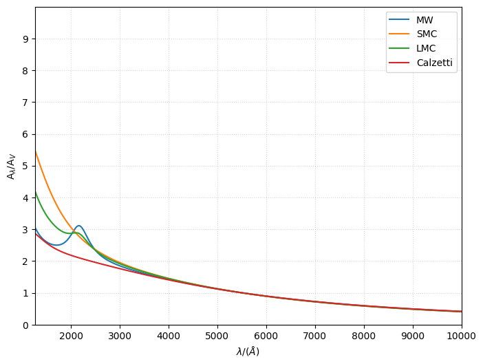
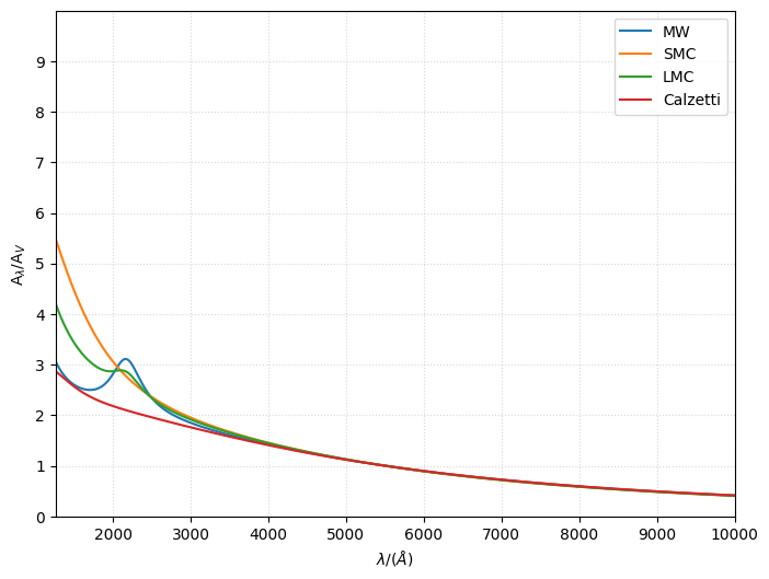
ParametricLi08
The ParametricLi08 model requires the UV slope (UV_slope, default 1.0), the optical to Near Infrared slope (OPT_NIR_slope, default 1.0), the Far UV slope (FUV_slope, default 1.0), and a dimensionless parameter between 0 and 1 controlling the strength of the UV bump (bump, default 0.0). Alternatively, a model string can be passed to adopt a preset model (possible values: "MW", "LMC", "SMC", or Calzetti).
[8]:
from synthesizer.emission_models.attenuation import ParametricLi08

mw_li08 = ParametricLi08(model="MW")
smc_li08 = ParametricLi08(model="SMC")
lmc_li08 = ParametricLi08(model="LMC")
calz_li08 = ParametricLi08(model="Calzetti")

fig, ax = mw_li08.plot_attenuation(lams, show=False, label="MW")
_, _ = smc_li08.plot_attenuation(lams, fig=fig, ax=ax, show=False, label="SMC")
_, _ = lmc_li08.plot_attenuation(lams, fig=fig, ax=ax, show=False, label="LMC")
_, _ = calz_li08.plot_attenuation(
    lams, fig=fig, ax=ax, show=False, label="Calzetti"
)
ax.grid(ls="dotted", alpha=0.5)
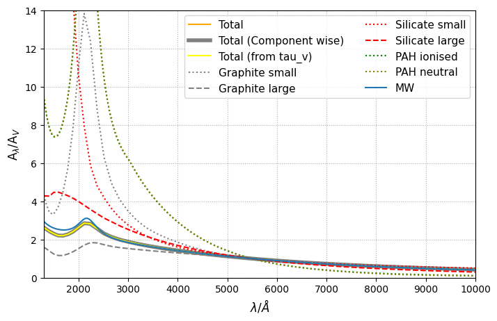
Draine and Li Extinction curve from grain size distribution
The DraineLiGrainCurves model gives the extinction curve for different grain species (Graphite, Silicate, PAH) based on the dust-to-gas ratio in small and large grains. Currently only two grain sizes are implemented for graphite and silicate, with one grain size (small grains) for PAHs. Default grids can be downloaded from the synthesizer grids box folder. The default grids have 0.01um and 0.1um as the small and large grain bin centres for graphite and silicate respectively, with the PAH bin
centre being 0.001um, all following a lognormal grain size distribution. Custom grids can be made by using the grid-generation package.
When using the model one should provide DraineLiGrainCurves with the required grain types and their bin centres in a dictionary, so that it knows beforehand these are the ones we want to look for. Obviously you should have made the dust grid beforehand with those choices that needs to be passed to the function.
To generate the optical depth the model requires one to specify the line-of-sight dust column density and the hydrogen column density in the grain components e.g. "graphite_a0p01um": 0.002 * Msun / pc**2 as shown below.
[9]:
import matplotlib.pyplot as plt
from unyt import Msun, pc

from synthesizer.units import DefaultUnits

default_units = DefaultUnits()

from synthesizer import GRID_DIR
from synthesizer.emission_models.attenuation import DraineLiGrainCurves

# Load our grid with the required properties
grid_dir = GRID_DIR
grid_name = "dust_extcurve_draine_li_lognormal_asmall0p01_alarge0p1_apah0p001"
# define the input grain properties
# we want to be using, this is in the
# format grain: bin centers
grain_dict = {
    "graphite": [0.01, 0.1],
    "silicate": [0.01, 0.1],
    "pahionised": [0.001],
    "pahneutral": [0.001],
}
dl_extcurve = DraineLiGrainCurves(
    lam=lams, grid_name=grid_name, grid_dir=grid_dir, grain_dict=grain_dict
)

# Define some of the dust grain properties we want to provide, the value has
# not much meaning other than the fact that they give dust-to-gas ratios in
# a reasonable range within the grid.
# Also note that the attenuation curve is determined by only the dust surface
# densities, sigmalos_H is there since the grid is defined in terms of
# dust-to-gas ratios. This makes sense as the attenuation should only
# depend on the dust along the line of sight, and not on the total gas
# or hydrogen mass.
sigmalos_H = 1000.0 * Msun / pc**2
sigmalos_dust = {
    "sigmalos_graphite_a0p01um": 0.001 * Msun / pc**2,
    "sigmalos_graphite_a0p1um": 0.005 * Msun / pc**2,
    "sigmalos_silicate_a0p01um": 0.001 * Msun / pc**2,
    "sigmalos_silicate_a0p1um": 0.005 * Msun / pc**2,
    "sigmalos_pahionised_a0p001um": 0.0001 * Msun / pc**2,
    "sigmalos_pahneutral_a0p001um": 0.0001 * Msun / pc**2,
}

Alam_g_small = dl_extcurve.get_tau_at_lam(
    lams,
    sigmalos_H=sigmalos_H,
    sigmalos_graphite_a0p01um=sigmalos_dust["sigmalos_graphite_a0p01um"],
)
Alam_g_large = dl_extcurve.get_tau_at_lam(
    lams,
    sigmalos_H=sigmalos_H,
    sigmalos_graphite_a0p1um=sigmalos_dust["sigmalos_graphite_a0p1um"],
)
Alam_s_small = dl_extcurve.get_tau_at_lam(
    lams,
    sigmalos_H=sigmalos_H,
    sigmalos_silicate_a0p01um=sigmalos_dust["sigmalos_silicate_a0p01um"],
)
Alam_s_large = dl_extcurve.get_tau_at_lam(
    lams,
    sigmalos_H=sigmalos_H,
    sigmalos_silicate_a0p1um=sigmalos_dust["sigmalos_silicate_a0p1um"],
)
Alam_pahion = dl_extcurve.get_tau_at_lam(
    lams,
    sigmalos_H=sigmalos_H,
    sigmalos_pahionised_a0p001um=sigmalos_dust["sigmalos_pahionised_a0p001um"],
)
Alam_pahneutral = dl_extcurve.get_tau_at_lam(
    lams,
    sigmalos_H=sigmalos_H,
    sigmalos_pahneutral_a0p001um=sigmalos_dust["sigmalos_pahneutral_a0p001um"],
)

Alam_tot = (
    Alam_g_small
    + Alam_g_large
    + Alam_s_small
    + Alam_s_large
    + Alam_pahion
    + Alam_pahneutral
)
Alam_tot_all = dl_extcurve.get_tau_at_lam(
    lams, sigmalos_H=sigmalos_H, **sigmalos_dust
)
Alam_tot_v = dl_extcurve.get_tau(
    lam=lams, sigmalos_H=sigmalos_H, **sigmalos_dust
)

fig, ax = plt.subplots(figsize=(8, 5))

ix = np.argmin(np.abs(lams - 5500 * Angstrom))
ax.plot(lams, Alam_tot_all / Alam_tot_all[ix], color="orange", label="Total")
ax.plot(
    lams,
    Alam_tot / Alam_tot[ix],
    color="black",
    label="Total (Component wise)",
    lw=4,
    alpha=0.5,
)
ax.plot(lams, Alam_tot_v, color="yellow", label="Total (from tau_v)")
ax.plot(
    lams,
    Alam_g_small / Alam_g_small[ix],
    color="grey",
    ls="dotted",
    label="Graphite small",
)
ax.plot(
    lams,
    Alam_g_large / Alam_g_large[ix],
    color="grey",
    ls="dashed",
    label="Graphite large",
)
ax.plot(
    lams,
    Alam_s_small / Alam_s_small[ix],
    color="red",
    ls="dotted",
    label="Silicate small",
)
ax.plot(
    lams,
    Alam_s_large / Alam_s_large[ix],
    color="red",
    ls="dashed",
    label="Silicate large",
)
ax.plot(
    lams,
    Alam_pahion / Alam_pahion[ix],
    color="green",
    ls="dotted",
    label="PAH ionised",
)
ax.plot(
    lams,
    Alam_pahneutral / Alam_pahneutral[ix],
    color="olive",
    ls="dotted",
    label="PAH neutral",
)

from synthesizer.emission_models.attenuation import ParametricLi08

MW_li08 = ParametricLi08(model="MW")
ax.plot(lams, MW_li08.get_tau(lam=lams), label="MW")

ax.set_xlim(1300, 10000)
ax.set_ylim(0, 14)
ax.set_ylabel(r"A$_{\lambda}$/A$_{V}$", fontsize=12)
ax.set_xlabel(r"$\lambda$/$\AA$", fontsize=12)
ax.grid(ls="dotted")
ax.legend(ncols=2, fontsize=11)

plt.show()
Varying Attenuation Law Parameters
The parameters of an attenuation law (e.g. the slope of a PowerLaw) can be varied on-the-fly when calculating the attenuation or transmission curves. This allows us to instantiate a single attenuation law object, and then vary its parameters as needed, e.g. for generating a population of galaxies with different attenuation law slopes.
The way this works in practice is that we instantiate the attenuation law emission model as normal, but we override the parameters we want to vary with a string input, which will be the argument the code looks for on the emission model and emitter.
[10]:
from synthesizer.emission_models.attenuation import ParametricLi08

dust_curve = ParametricLi08(
    model="MW",
    OPT_NIR_slope="optical_slope",
    UV_slope="uv_slp",
    FUV_slope=None,
    bump="bump_ampl",
)
This emission model is not useable on its own, but when attached to a parent EmissionModel or emitter with the appropriate parameters, the parameters will be overridden on-the-fly when calculating the attenuation or transmission curves.
In the below example, we instantiate a ParametricLi08 attenuation law, but override the OPT_NIR_slope, UV_slope, and bump parameters with strings. When this attenuation law is attached to an emitter or emission model with these parameters, the values will be used instead of the defaults. If you set a parameter to None, it will expect an override with the same name as the parameter (e.g. FUV_slope in this case).
[11]:
from unyt import Msun, yr
from synthesizer.emission_models import TotalEmission
from synthesizer.grid import Grid
from synthesizer.parametric import Stars
grid = Grid("test_grid.hdf5")
stars = Stars(
log10ages=grid.log10ages,
metallicities=grid.metallicities,
sf_hist=1e6 * yr,
metal_dist=0.02,
initial_mass=1e8 * Msun,
optical_slope=-0.7,
uv_slp=3.0,
tau_v=1.0,
)
emergent = TotalEmission(
grid=grid, dust_curve=dust_curve, bump_ampl=10, FUV_slope=2.0
)
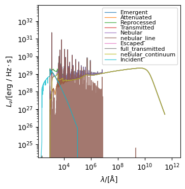
stars.get_spectra(emergent)
stars.plot_spectra()
[11]:
(<Figure size 350x500 with 1 Axes>,
 <Axes: xlabel='$\\lambda/[\\mathrm{\\AA}]$', ylabel='$L_{\\nu}/[\\mathrm{\\rm{erg} \\ / \\ \\rm{Hz \\cdot \\rm{s}}}]$'>)