Black Hole Spectra

Black hole spectra can be generated by combining a BlackHoles (for particle, BlackHole for parametric) object with an EmissionModel, translating the physical properties of the blackhole(s) (e.g. mass, accretion_rate, etc.) to a spectral energy distribution.

These models are described in detail in the emission model docs. Here, we’ll use an instance of a UnifiedAGN model for demonstration purposes.

The following sections demonstrate the generation of combined spectra (which is the same for both parametric and particle BlackHoles) and per-particle spectra.

import numpy as np
from unyt import K, Mpc, Msun, cm, deg, yr

from synthesizer import Grid
from synthesizer.emission_models import (
    Greybody,
    UnifiedAGN,
)
from synthesizer.emission_models.attenuation import PowerLaw
from synthesizer.parametric import BlackHole

# Get the NLR and BLR grids
nlr_grid = Grid("test_grid_agn-nlr")
blr_grid = Grid("test_grid_agn-blr")


# Initialise the BlackHole object setting most of the key attributes
blackhole = BlackHole(
    mass=1e8 * Msun,
    inclination=60 * deg,
    accretion_rate_eddington=0.1,
    covering_fraction_nlr=0.1,
    covering_fraction_blr=0.1,
    metallicity=0.01,
    theta_torus=20 * deg,
)

# Initialise the UnifiedAGN model
uniagn = UnifiedAGN(
    nlr_grid,
    blr_grid,
    ionisation_parameter_nlr=0.01,
    hydrogen_density_nlr=1e4 * cm**-3,
    ionisation_parameter_blr=0.1,
    hydrogen_density_blr=1e10 * cm**-3,
    torus_emission_model=Greybody(1000 * K, 1.5),
)

Integrated spectra

To generate integrated spectra we simply call the component’s get_spectra method. This method will populate the component’s spectra attribute with a dictionary containing Sed objects for each spectra in the EmissionModel. It will also return the spectra at the root of the EmissionModel.

# Get the spectra using a unified agn model (instantiated elsewhere)
spectra = blackhole.get_spectra(uniagn)

fig, ax = blackhole.plot_spectra(
    show=True, ylimits=(10**27.5, 10**34.0), figsize=(6, 4)
)

/opt/hostedtoolcache/Python/3.10.19/x64/lib/python3.10/site-packages/unyt/array.py:1832: RuntimeWarning: overflow encountered in exp
  out_arr = func(np.asarray(inp), out=out_func, **kwargs)
/opt/hostedtoolcache/Python/3.10.19/x64/lib/python3.10/site-packages/unyt/array.py:1972: RuntimeWarning: overflow encountered in multiply
  out_arr = func(

Including dust attenuation

We can also generate spectra including attenuation and emission from diffuse dust along the line of sight to the black hole. This is now possible directly with the UnifiedAGN by passing a dust curve. The optical depth (tau_v) must be available on the emitter (the blackhole) or set by the emission model.

tau_v = 0.5

# Initialise the UnifiedAGN model
uniagn_attenuated = UnifiedAGN(
    nlr_grid,
    blr_grid,
    ionisation_parameter_nlr=0.01,
    hydrogen_density_nlr=1e4 * cm**-3,
    ionisation_parameter_blr=0.1,
    hydrogen_density_blr=1e10 * cm**-3,
    torus_emission_model=Greybody(1000 * K, 1.5),
    diffuse_dust_curve=PowerLaw(slope=-1.0),
    tau_v=tau_v,
)

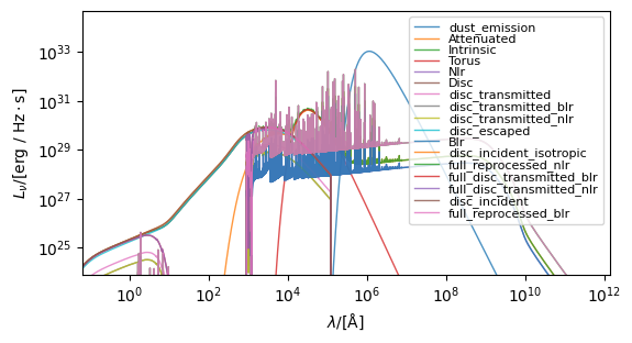
We then follow the same process of calling get_spectra with the new model. The plot here shows luminosity rather than spectral energy density.

spectra = blackhole.get_spectra(uniagn_attenuated)

fig, ax = blackhole.plot_spectra(
    quantity_to_plot="luminosity",
    figsize=(6, 4),
    spectra_to_plot=["intrinsic", "attenuated"],
)

The spectra returned by get_spectra is the “dust_emission” spectra at the root of the emission model.

print(spectra)

+-------------------------------------------------------------------------------------------------+
|                                               SED                                               |
+---------------------------+---------------------------------------------------------------------+
| Attribute                 | Value                                                               |
+---------------------------+---------------------------------------------------------------------+
| redshift                  | 0                                                                   |
+---------------------------+---------------------------------------------------------------------+
| ndim                      | 1                                                                   |
+---------------------------+---------------------------------------------------------------------+
| nlam                      | 9244                                                                |
+---------------------------+---------------------------------------------------------------------+
| shape                     | (9244,)                                                             |
+---------------------------+---------------------------------------------------------------------+
| lam (9244,)               | 1.30e-04 Å -> 2.99e+11 Å (Mean: 9.73e+09 Å)                         |
+---------------------------+---------------------------------------------------------------------+
| nu (9244,)                | 1.00e+07 Hz -> 2.31e+22 Hz (Mean: 8.51e+19 Hz)                      |
+---------------------------+---------------------------------------------------------------------+
| lnu (9244,)               | 0.00e+00 erg/(Hz*s) -> 1.45e+31 erg/(Hz*s) (Mean: 1.12e+29 erg)     |
+---------------------------+---------------------------------------------------------------------+
| bolometric_luminosity     | 3.851157354809097e+44 erg/s                                         |
+---------------------------+---------------------------------------------------------------------+
| energy (9244,)            | 4.14e-08 eV -> 9.56e+07 eV (Mean: 3.52e+05 eV)                      |
+---------------------------+---------------------------------------------------------------------+
| frequency (9244,)         | 1.00e+07 Hz -> 2.31e+22 Hz (Mean: 8.51e+19 Hz)                      |
+---------------------------+---------------------------------------------------------------------+
| llam (9244,)              | 0.00e+00 erg/(s*Å) -> 3.59e+41 erg/(s*Å) (Mean: 1.97e+39 erg/(s*Å)) |
+---------------------------+---------------------------------------------------------------------+
| luminosity (9244,)        | 0.00e+00 erg/s -> 1.80e+45 erg/s (Mean: 1.25e+43 erg/s)             |
+---------------------------+---------------------------------------------------------------------+
| luminosity_lambda (9244,) | 0.00e+00 erg/(s*Å) -> 3.59e+41 erg/(s*Å) (Mean: 1.97e+39 erg/(s*Å)) |
+---------------------------+---------------------------------------------------------------------+
| luminosity_nu (9244,)     | 0.00e+00 erg/(Hz*s) -> 1.45e+31 erg/(Hz*s) (Mean: 1.12e+29 erg)     |
+---------------------------+---------------------------------------------------------------------+
| wavelength (9244,)        | 1.30e-04 Å -> 2.99e+11 Å (Mean: 9.73e+09 Å)                         |
+---------------------------+---------------------------------------------------------------------+

However, all the spectra are stored within a dictionary under the spectra attribute.

print(blackhole.spectra)

{'disc_incident_isotropic': <synthesizer.emissions.sed.Sed object at 0x7f5f12398340>, 'full_reprocessed_nlr': <synthesizer.emissions.sed.Sed object at 0x7f5f12367610>, 'full_reprocessed_blr': <synthesizer.emissions.sed.Sed object at 0x7f5f12367670>, 'disc_incident_masked': <synthesizer.emissions.sed.Sed object at 0x7f5f12398220>, 'disc_transmitted_nlr_full': <synthesizer.emissions.sed.Sed object at 0x7f5f123982b0>, 'disc_transmitted_blr_full': <synthesizer.emissions.sed.Sed object at 0x7f5f123675e0>, 'disc_incident': <synthesizer.emissions.sed.Sed object at 0x7f5f123983d0>, 'disc_transmitted_blr_isotropic_full': <synthesizer.emissions.sed.Sed object at 0x7f5f12398460>, 'disc_transmitted_nlr_isotropic_full': <synthesizer.emissions.sed.Sed object at 0x7f5f123984f0>, 'full_continuum_blr': <synthesizer.emissions.sed.Sed object at 0x7f5f12398580>, 'full_continuum_nlr': <synthesizer.emissions.sed.Sed object at 0x7f5f12367be0>, 'torus': <synthesizer.emissions.sed.Sed object at 0x7f5f123673a0>, 'nlr': <synthesizer.emissions.sed.Sed object at 0x7f5f12398c40>, 'blr': <synthesizer.emissions.sed.Sed object at 0x7f5f123982e0>, 'disc_escaped': <synthesizer.emissions.sed.Sed object at 0x7f5f123980d0>, 'disc_transmitted_nlr': <synthesizer.emissions.sed.Sed object at 0x7f5f12398070>, 'disc_transmitted_blr': <synthesizer.emissions.sed.Sed object at 0x7f5f12398520>, 'disc_transmitted': <synthesizer.emissions.sed.Sed object at 0x7f5f13f47af0>, 'disc': <synthesizer.emissions.sed.Sed object at 0x7f5f12367310>, 'disc_transmitted_blr_isotropic': <synthesizer.emissions.sed.Sed object at 0x7f5f12398e20>, 'disc_escaped_isotropic': <synthesizer.emissions.sed.Sed object at 0x7f5f12398490>, 'disc_transmitted_nlr_isotropic': <synthesizer.emissions.sed.Sed object at 0x7f5f12398d30>, 'disc_averaged_without_torus': <synthesizer.emissions.sed.Sed object at 0x7f5f12367c40>, 'disc_averaged': <synthesizer.emissions.sed.Sed object at 0x7f5f12398c70>, 'blr_continuum': <synthesizer.emissions.sed.Sed object at 0x7f5f123986d0>, 'line_regions': <synthesizer.emissions.sed.Sed object at 0x7f5f12398cd0>, 'disc_transmitted_blr_weighted': <synthesizer.emissions.sed.Sed object at 0x7f5f123985e0>, 'disc_transmitted_nlr_weighted': <synthesizer.emissions.sed.Sed object at 0x7f5f123985b0>, 'disc_escaped_weighted': <synthesizer.emissions.sed.Sed object at 0x7f5f12398d00>, 'disc_transmitted_weighted_combination': <synthesizer.emissions.sed.Sed object at 0x7f5f12398e80>, 'nlr_continuum': <synthesizer.emissions.sed.Sed object at 0x7f5f12399000>, 'intrinsic': <synthesizer.emissions.sed.Sed object at 0x7f5f12367850>, 'attenuated': <synthesizer.emissions.sed.Sed object at 0x7f5f12398c10>}

Particle spectra

To demonstrate the particle spectra functionality we first generate some mock particle black hole data, and initialise a BlackHoles object.

from synthesizer.particle import BlackHoles

# Make fake properties
n = 4
masses = 10 ** np.random.uniform(low=7, high=9, size=n) * Msun
coordinates = np.random.normal(0, 1.5, (n, 3)) * Mpc
accretion_rates = 10 ** np.random.uniform(low=-2, high=1, size=n) * Msun / yr
metallicities = np.full(n, 0.01)

# And get the black holes object
blackholes = BlackHoles(
    masses=masses,
    coordinates=coordinates,
    accretion_rates=accretion_rates,
    metallicities=metallicities,
    ionisation_parameter_nlr=0.01,
    hydrogen_density_nlr=1e4 * cm**-3,
    ionisation_parameter_blr=0.1,
    hydrogen_density_blr=1e10 * cm**-3,
)

To generate a spectra for each black hole (per particle) we use the same emission model, but we need to tell the model to produce a spectrum for each particle. This is done by setting the per_particle flag to True on the model.

uniagn_attenuated.set_per_particle(True)

With that done we just call the same get_spectra method on the component, and the particle spectra will be stored in the particle_spectra attribute of the component.

spectra = blackholes.get_spectra(uniagn_attenuated, verbose=True)

Again, the returned spectra is the “dust_emission” spectra from the root of the model.

print(spectra)

+---------------------------------------------------------------------------------------------------+
|                                                SED                                                |
+-----------------------------+---------------------------------------------------------------------+
| Attribute                   | Value                                                               |
+-----------------------------+---------------------------------------------------------------------+
| redshift                    | 0                                                                   |
+-----------------------------+---------------------------------------------------------------------+
| ndim                        | 2                                                                   |
+-----------------------------+---------------------------------------------------------------------+
| nlam                        | 9244                                                                |
+-----------------------------+---------------------------------------------------------------------+
| shape                       | (4, 9244)                                                           |
+-----------------------------+---------------------------------------------------------------------+
| lam (9244,)                 | 1.30e-04 Å -> 2.99e+11 Å (Mean: 9.73e+09 Å)                         |
+-----------------------------+---------------------------------------------------------------------+
| nu (9244,)                  | 1.00e+07 Hz -> 2.31e+22 Hz (Mean: 8.51e+19 Hz)                      |
+-----------------------------+---------------------------------------------------------------------+
| lnu (4, 9244)               | 0.00e+00 erg/(Hz*s) -> 3.39e+32 erg/(Hz*s) (Mean: 6.80e+29 erg)     |
+-----------------------------+---------------------------------------------------------------------+
| bolometric_luminosity (4,)  | 7.34e+43 erg/s -> 1.05e+46 erg/s (Mean: 2.82e+45 erg/s)             |
+-----------------------------+---------------------------------------------------------------------+
| energy (9244,)              | 4.14e-08 eV -> 9.56e+07 eV (Mean: 3.52e+05 eV)                      |
+-----------------------------+---------------------------------------------------------------------+
| frequency (9244,)           | 1.00e+07 Hz -> 2.31e+22 Hz (Mean: 8.51e+19 Hz)                      |
+-----------------------------+---------------------------------------------------------------------+
| llam (4, 9244)              | 0.00e+00 erg/(s*Å) -> 7.75e+42 erg/(s*Å) (Mean: 1.96e+40 erg/(s*Å)) |
+-----------------------------+---------------------------------------------------------------------+
| luminosity (4, 9244)        | 0.00e+00 erg/s -> 3.89e+46 erg/s (Mean: 9.14e+43 erg/s)             |
+-----------------------------+---------------------------------------------------------------------+
| luminosity_lambda (4, 9244) | 0.00e+00 erg/(s*Å) -> 7.75e+42 erg/(s*Å) (Mean: 1.96e+40 erg/(s*Å)) |
+-----------------------------+---------------------------------------------------------------------+
| luminosity_nu (4, 9244)     | 0.00e+00 erg/(Hz*s) -> 3.39e+32 erg/(Hz*s) (Mean: 6.80e+29 erg)     |
+-----------------------------+---------------------------------------------------------------------+
| wavelength (9244,)          | 1.30e-04 Å -> 2.99e+11 Å (Mean: 9.73e+09 Å)                         |
+-----------------------------+---------------------------------------------------------------------+

While the spectra produced by get_particle_spectra are stored in a dictionary under the particle_spectra attribute.

print(blackholes.particle_spectra)

{'full_reprocessed_blr': <synthesizer.emissions.sed.Sed object at 0x7f5f123eab30>, 'full_reprocessed_nlr': <synthesizer.emissions.sed.Sed object at 0x7f5f1249da50>, 'disc_transmitted_blr_full': <synthesizer.emissions.sed.Sed object at 0x7f5f123999c0>, 'disc_incident_masked': <synthesizer.emissions.sed.Sed object at 0x7f5f1249fb80>, 'disc_transmitted_nlr_full': <synthesizer.emissions.sed.Sed object at 0x7f5f1021da50>, 'disc_incident_isotropic': <synthesizer.emissions.sed.Sed object at 0x7f5f12399c30>, 'disc_incident': <synthesizer.emissions.sed.Sed object at 0x7f5f123eb310>, 'disc_transmitted_blr_isotropic_full': <synthesizer.emissions.sed.Sed object at 0x7f5f123eb190>, 'disc_transmitted_nlr_isotropic_full': <synthesizer.emissions.sed.Sed object at 0x7f5f123eb5b0>, 'full_continuum_blr': <synthesizer.emissions.sed.Sed object at 0x7f5f123e98a0>, 'full_continuum_nlr': <synthesizer.emissions.sed.Sed object at 0x7f5f123e8c10>, 'blr': <synthesizer.emissions.sed.Sed object at 0x7f5f124163e0>, 'nlr': <synthesizer.emissions.sed.Sed object at 0x7f5f124174c0>, 'disc_transmitted_blr': <synthesizer.emissions.sed.Sed object at 0x7f5f10201120>, 'disc_escaped': <synthesizer.emissions.sed.Sed object at 0x7f5f10202320>, 'disc_transmitted_nlr': <synthesizer.emissions.sed.Sed object at 0x7f5f12415990>, 'disc_transmitted': <synthesizer.emissions.sed.Sed object at 0x7f5f10202140>, 'disc': <synthesizer.emissions.sed.Sed object at 0x7f5f12415540>, 'torus': <synthesizer.emissions.sed.Sed object at 0x7f5f12417550>, 'line_regions': <synthesizer.emissions.sed.Sed object at 0x7f5f124144c0>, 'disc_transmitted_blr_isotropic': <synthesizer.emissions.sed.Sed object at 0x7f5f12414970>, 'disc_escaped_isotropic': <synthesizer.emissions.sed.Sed object at 0x7f5f12417430>, 'disc_transmitted_nlr_isotropic': <synthesizer.emissions.sed.Sed object at 0x7f5f12414a60>, 'disc_averaged_without_torus': <synthesizer.emissions.sed.Sed object at 0x7f5f12414730>, 'disc_averaged': <synthesizer.emissions.sed.Sed object at 0x7f5f12416890>, 'blr_continuum': <synthesizer.emissions.sed.Sed object at 0x7f5f12417850>, 'disc_transmitted_blr_weighted': <synthesizer.emissions.sed.Sed object at 0x7f5f12417af0>, 'disc_transmitted_nlr_weighted': <synthesizer.emissions.sed.Sed object at 0x7f5f124149a0>, 'disc_escaped_weighted': <synthesizer.emissions.sed.Sed object at 0x7f5f12414640>, 'disc_transmitted_weighted_combination': <synthesizer.emissions.sed.Sed object at 0x7f5f124144f0>, 'nlr_continuum': <synthesizer.emissions.sed.Sed object at 0x7f5f12416a70>, 'intrinsic': <synthesizer.emissions.sed.Sed object at 0x7f5f12414a00>, 'attenuated': <synthesizer.emissions.sed.Sed object at 0x7f5f12416ad0>}

Integrating spectra

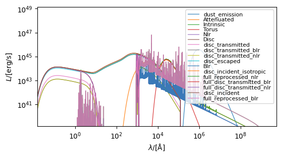
The integrated spectra are automatically produced alongside per particle spectra. However, if we wanted to explictly get the integrated spectra from the particle spectra we just generated (for instance if we had made some modification after generation), we can call the integrate_particle_spectra method. This method will sum the individual spectra and populate the spectra dictionary.

Note, we can also integrate individual spectra using the Sed.sum() method.

print(blackholes.spectra)
blackholes.integrate_particle_spectra()
print(blackholes.spectra)

fig, ax = blackholes.plot_spectra(show=True, figsize=(6, 4))

{'full_reprocessed_blr': <synthesizer.emissions.sed.Sed object at 0x7f5f123ea2c0>, 'full_reprocessed_nlr': <synthesizer.emissions.sed.Sed object at 0x7f5f123676a0>, 'disc_transmitted_blr_full': <synthesizer.emissions.sed.Sed object at 0x7f5f1021cb20>, 'disc_incident_masked': <synthesizer.emissions.sed.Sed object at 0x7f5f123e9570>, 'disc_transmitted_nlr_full': <synthesizer.emissions.sed.Sed object at 0x7f5f123e9720>, 'disc_incident_isotropic': <synthesizer.emissions.sed.Sed object at 0x7f5f123eb370>, 'disc_incident': <synthesizer.emissions.sed.Sed object at 0x7f5f123ebee0>, 'disc_transmitted_blr_isotropic_full': <synthesizer.emissions.sed.Sed object at 0x7f5f123e8c70>, 'disc_transmitted_nlr_isotropic_full': <synthesizer.emissions.sed.Sed object at 0x7f5f123e9750>, 'full_continuum_blr': <synthesizer.emissions.sed.Sed object at 0x7f5f123e8490>, 'full_continuum_nlr': <synthesizer.emissions.sed.Sed object at 0x7f5f123e8100>, 'blr': <synthesizer.emissions.sed.Sed object at 0x7f5f123e82b0>, 'nlr': <synthesizer.emissions.sed.Sed object at 0x7f5f123e9870>, 'disc_transmitted_blr': <synthesizer.emissions.sed.Sed object at 0x7f5f123e8ca0>, 'disc_escaped': <synthesizer.emissions.sed.Sed object at 0x7f5f123e8310>, 'disc_transmitted_nlr': <synthesizer.emissions.sed.Sed object at 0x7f5f102022c0>, 'disc_transmitted': <synthesizer.emissions.sed.Sed object at 0x7f5f12415c30>, 'disc': <synthesizer.emissions.sed.Sed object at 0x7f5f12416980>, 'torus': <synthesizer.emissions.sed.Sed object at 0x7f5f12417820>, 'line_regions': <synthesizer.emissions.sed.Sed object at 0x7f5f123e89d0>, 'disc_transmitted_blr_isotropic': <synthesizer.emissions.sed.Sed object at 0x7f5f123e8670>, 'disc_escaped_isotropic': <synthesizer.emissions.sed.Sed object at 0x7f5f12416740>, 'disc_transmitted_nlr_isotropic': <synthesizer.emissions.sed.Sed object at 0x7f5f124168f0>, 'disc_averaged_without_torus': <synthesizer.emissions.sed.Sed object at 0x7f5f12416320>, 'disc_averaged': <synthesizer.emissions.sed.Sed object at 0x7f5f12416ec0>, 'blr_continuum': <synthesizer.emissions.sed.Sed object at 0x7f5f124146d0>, 'disc_transmitted_blr_weighted': <synthesizer.emissions.sed.Sed object at 0x7f5f124151b0>, 'disc_transmitted_nlr_weighted': <synthesizer.emissions.sed.Sed object at 0x7f5f124172b0>, 'disc_escaped_weighted': <synthesizer.emissions.sed.Sed object at 0x7f5f12415060>, 'disc_transmitted_weighted_combination': <synthesizer.emissions.sed.Sed object at 0x7f5f12414c70>, 'nlr_continuum': <synthesizer.emissions.sed.Sed object at 0x7f5f12415330>, 'intrinsic': <synthesizer.emissions.sed.Sed object at 0x7f5f12415000>, 'attenuated': <synthesizer.emissions.sed.Sed object at 0x7f5f124157e0>}
{'full_reprocessed_blr': <synthesizer.emissions.sed.Sed object at 0x7f5f123ebb50>, 'full_reprocessed_nlr': <synthesizer.emissions.sed.Sed object at 0x7f5f12367520>, 'disc_transmitted_blr_full': <synthesizer.emissions.sed.Sed object at 0x7f5f123ea2c0>, 'disc_incident_masked': <synthesizer.emissions.sed.Sed object at 0x7f5f123e9060>, 'disc_transmitted_nlr_full': <synthesizer.emissions.sed.Sed object at 0x7f5f123e9570>, 'disc_incident_isotropic': <synthesizer.emissions.sed.Sed object at 0x7f5f123e9720>, 'disc_incident': <synthesizer.emissions.sed.Sed object at 0x7f5f123eb370>, 'disc_transmitted_blr_isotropic_full': <synthesizer.emissions.sed.Sed object at 0x7f5f123ebee0>, 'disc_transmitted_nlr_isotropic_full': <synthesizer.emissions.sed.Sed object at 0x7f5f123e8c70>, 'full_continuum_blr': <synthesizer.emissions.sed.Sed object at 0x7f5f123e9750>, 'full_continuum_nlr': <synthesizer.emissions.sed.Sed object at 0x7f5f123e8490>, 'blr': <synthesizer.emissions.sed.Sed object at 0x7f5f123e8100>, 'nlr': <synthesizer.emissions.sed.Sed object at 0x7f5f123e82b0>, 'disc_transmitted_blr': <synthesizer.emissions.sed.Sed object at 0x7f5f123e9870>, 'disc_escaped': <synthesizer.emissions.sed.Sed object at 0x7f5f123e8ca0>, 'disc_transmitted_nlr': <synthesizer.emissions.sed.Sed object at 0x7f5f123e8310>, 'disc_transmitted': <synthesizer.emissions.sed.Sed object at 0x7f5f102022c0>, 'disc': <synthesizer.emissions.sed.Sed object at 0x7f5f1249cfa0>, 'torus': <synthesizer.emissions.sed.Sed object at 0x7f5f12625510>, 'line_regions': <synthesizer.emissions.sed.Sed object at 0x7f5f10180520>, 'disc_transmitted_blr_isotropic': <synthesizer.emissions.sed.Sed object at 0x7f5f123676a0>, 'disc_escaped_isotropic': <synthesizer.emissions.sed.Sed object at 0x7f5f123e89d0>, 'disc_transmitted_nlr_isotropic': <synthesizer.emissions.sed.Sed object at 0x7f5f123e8670>, 'disc_averaged_without_torus': <synthesizer.emissions.sed.Sed object at 0x7f5f1021cb20>, 'disc_averaged': <synthesizer.emissions.sed.Sed object at 0x7f5f1021cac0>, 'blr_continuum': <synthesizer.emissions.sed.Sed object at 0x7f5f1249cd90>, 'disc_transmitted_blr_weighted': <synthesizer.emissions.sed.Sed object at 0x7f5f12416320>, 'disc_transmitted_nlr_weighted': <synthesizer.emissions.sed.Sed object at 0x7f5f124146d0>, 'disc_escaped_weighted': <synthesizer.emissions.sed.Sed object at 0x7f5f124151b0>, 'disc_transmitted_weighted_combination': <synthesizer.emissions.sed.Sed object at 0x7f5f124172b0>, 'nlr_continuum': <synthesizer.emissions.sed.Sed object at 0x7f5f12415060>, 'intrinsic': <synthesizer.emissions.sed.Sed object at 0x7f5f12414c70>, 'attenuated': <synthesizer.emissions.sed.Sed object at 0x7f5f12415330>}

Modifying EmissionModel parameters with get_spectra

As well as modifying a model explicitly, it’s also possible to override the properties of a model at the point get_spectra is called. These modifications will not be remembered by the model afterwards. As it stands, this form of modification is supported for the dust_curve, tau_v, covering_fraction and masks.

Here we’ll demonstrate this by overriding the covering fractions to generate spectra for a range of covering_fraction values. This can either be done by passing a single number which will overide all covering fractions on every model (probably undesirable behaviour since this will set NLR and BLR covering fractions to be equal).

# Since we now want integrated spectra lets remove the per particle flag
uniagn_attenuated.set_per_particle(False)

blackhole.clear_all_spectra()
spectra = {}
for fesc in [0.1, 0.5, 0.9]:
    blackhole.get_spectra(uniagn_attenuated, covering_fraction=fesc)
    spectra[r"$f " f"=$ {fesc}"] = blackhole.spectra["intrinsic"]

Or (more desirably) we can pass a dictionary mapping model labels to fesc values to target specific models. Notice that we have invoked the clear_all_spectra method to reset the spectra dictionary, we can also clear all emissions (including spectra, lines, and photometry if they are present) with the clear_all_emissions method.

blackhole.clear_all_emissions()
spectra = {}
for nlr_fesc in [0.1, 0.5, 0.9]:
    for blr_fesc in [0.1, 0.5, 0.9]:
        if nlr_fesc + blr_fesc > 1:
            continue
        blackhole.get_spectra(
            uniagn_attenuated,
            covering_fraction={
                "disc_transmitted_nlr": nlr_fesc,
                "disc_transmitted_blr": blr_fesc,
            },
        )
        spectra[
            r"$f_\mathrm{nlr} "
            f"=$ {nlr_fesc}, "
            r"$f_\mathrm{blr} "
            f"=$ {blr_fesc},"
        ] = blackhole.spectra["intrinsic"]

To see the variation above we can pass the dictionary we populated with the varied spectra to the plot_spectra function (where the dictionary keys will be used as labels).

from synthesizer.emissions import plot_spectra

plot_spectra(
    spectra,
    figsize=(8, 4),
    ylimits=(10**29.0, 10**34.0),
    xlimits=(9 * 10**2, 10**4),
    show=True,
)

(<Figure size 800x400 with 1 Axes>,
 <Axes: xlabel='$\\lambda/[\\mathrm{\\AA}]$', ylabel='$L_{\\nu}/[\\mathrm{\\rm{erg} \\ / \\ \\rm{Hz \\cdot \\rm{s}}}]$'>)