Dust emission

Synthesizer can model thermal dust emission using different approaches and generators. This is done using dust emission models, which can then be handed to an EmissionModel to produce a dust emission spectrum, which can be combined with any other spectra in the model.

Dust emission generators come in two main types:

• Energy Balance: Models that calculate dust luminosity from the energy absorbed by dust (difference between intrinsic and attenuated stellar emission)

• Scaler: Models that scale a normalized dust spectrum by the bolometric luminosity of another emission component

First we load some common modules, and define a wavelength array over which we will generate our dust emission SED

import matplotlib.pyplot as plt
import numpy as np
from unyt import Angstrom, K, Lsun, Msun, um

from synthesizer.emission_models.generators.dust import (
    Blackbody,
    Casey12,
    DraineLi07,
    Greybody,
)

lam = 10 ** (np.arange(3.0, 8.0, 0.01)) * Angstrom

Energy Balance vs Scaler Emission Types

Before exploring specific dust models, it’s important to understand the two fundamental approaches for dust emission in Synthesizer:

Energy Balance Dust Emission

Energy balance models calculate the dust luminosity from the energy absorbed by dust. This is done by taking the difference between the intrinsic (unattenuated) and attenuated stellar emission:

L_dust = L_intrinsic - L_attenuated

This approach is physically motivated as it conserves energy: the energy absorbed by dust should equal the energy re-emitted in the infrared.

Scaler Dust Emission

Scaler models normalize a dust emission spectrum and then scale it by the bolometric luminosity of another emission component. This provides more flexibility in defining how the dust emission relates to other galaxy components.

Most examples below use the get_spectra method directly on the generators to show their spectral shapes, but in practice these generators are typically used within EmissionModel instances.

Blackbody Dust Emission

The simplest dust emission model is a blackbody, which follows Planck’s law for thermal emission. This represents optically thick dust emission where the emissivity is unity at all wavelengths.

The blackbody generator is useful for:

• Simple thermal dust modeling

• Quick approximations when detailed dust properties are unknown

• Baseline comparisons with more complex models

Below we show blackbody spectra for different temperatures:

for T in [10, 25, 50, 100, 200]:
    model = Blackbody(temperature=T * K)
    sed = model.get_spectra(lam)
    plt.loglog(sed.lam, sed.luminosity, label=f"T={T} K")

plt.title("Blackbody Dust Emission")
plt.xlabel(r"$ \lambda / \AA$")
plt.ylabel(r"$ L_{\nu} / L_{bol}$")
plt.xlim(1e4, 1e8)
plt.ylim(10**-3.0, 1.5)
plt.legend()
plt.show()

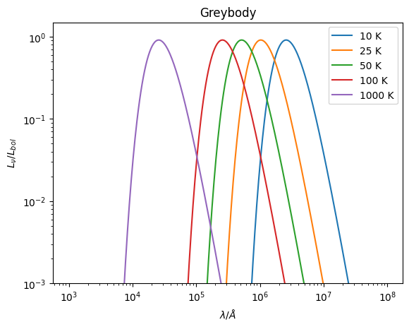
Greybody Dust Emission

A greybody model extends the blackbody by including wavelength-dependent emissivity. This is more realistic for astronomical dust, which often has emissivity that varies with wavelength according to a power law.

Key features of the greybody model:

• Emissivity index: Controls how emissivity varies with wavelength (typically β = 1-2 for astronomical dust)

• Optically thin/thick transition: Can model the transition from optically thick to thin emission

• Reference wavelength: Wavelength where the optical depth transition occurs

The greybody emission follows: ε(λ) ∝ (λ_0/λ)^β for the optically thin case, where λ_0 is the reference wavelength and β is the emissivity index.

Below we show greybody spectra for optically thin (solid lines) and optically thick (dashed lines) cases:

for ii, T in enumerate([25, 50, 100, 200]):
    color = plt.cm.tab10(ii)
    # Optically thin
    model = Greybody(temperature=T * K, emissivity=2.0, optically_thin=True)
    sed = model.get_spectra(lam)
    plt.loglog(sed.lam, sed.luminosity, label=f"T={T} K", color=color)

    # Optically thick below 100um
    model = Greybody(
        temperature=T * K, emissivity=2.0, lam_0=100 * um, optically_thin=False
    )
    sed = model.get_spectra(lam)
    plt.loglog(sed.lam, sed.luminosity, ls="dashed", color=color)

plt.title("Greybody Dust Emission")
plt.xlabel(r"$ \lambda / \AA$")
plt.ylabel(r"$ L_{\nu} / L_{bol}$")
plt.xlim(1e4, 1e8)
plt.ylim(10**-3.0, 1.5)
plt.legend()
plt.show()

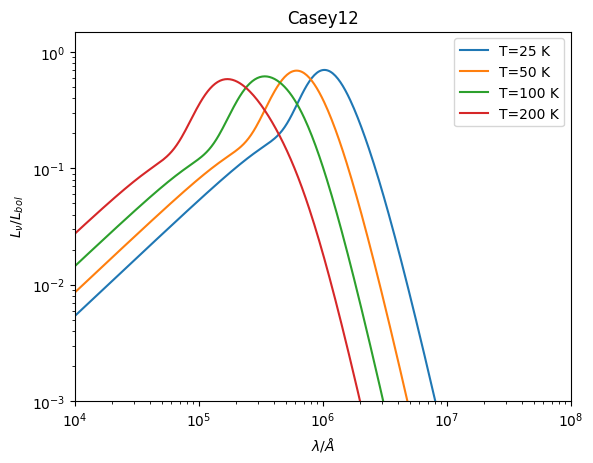
Casey12 Dust Emission

The Casey12 model follows Casey (2012) and combines a mid-infrared power law with a far-infrared greybody component. This model is particularly useful for modeling galaxy SEDs where both warm (mid-IR) and cold (far-IR) dust components contribute.

Key features of the Casey12 model:

• Mid-IR power law: Follows L_ν ∝ ν^α for λ < λ_0

• Far-IR greybody: Modified blackbody emission for λ > λ_0

• Smooth transition: The model smoothly transitions between the two regimes at λ_0

• Temperature and emissivity: Controls the far-IR peak and slope

The model provides a good empirical fit to observed galaxy SEDs, especially for star-forming galaxies with significant dust heating.

Below we show Casey12 spectra for different temperatures:

for ii, T in enumerate([25, 50, 100, 200]):
    color = plt.cm.tab10(ii)
    model = Casey12(
        temperature=T * K, emissivity=2.0, alpha=2.0, lam_0=100 * um
    )
    sed = model.get_spectra(lam)
    plt.loglog(sed.lam, sed.luminosity, label=f"T={T} K", color=color)

plt.title("Casey12 Dust Emission")
plt.xlabel(r"$ \lambda / \AA$")
plt.ylabel(r"$ L_{\nu} / L_{bol}$")
plt.xlim(1e4, 1e8)
plt.ylim(10**-3.0, 1.5)
plt.legend()
plt.show()

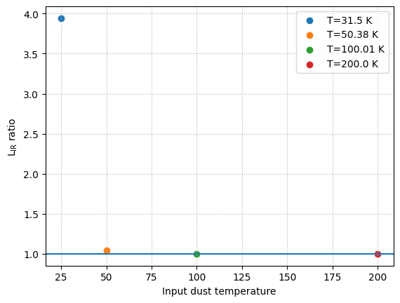
CMB Heating Effects

At high redshift, the effect of CMB heating becomes important for dust emission. The cosmic microwave background temperature increases as T_CMB(z) = T_CMB(0) × (1 + z), providing an additional heating source for dust grains.

To account for this, any dust emission model can incorporate CMB heating by setting cmb_heating=True and providing a redshift. This modifies both the effective dust temperature and the total infrared luminosity.

Below we compare the Casey12 model with and without CMB heating at z=10:

for ii, T in enumerate([25, 50, 100, 200]):
    color = plt.cm.tab10(ii)
    model = Casey12(
        temperature=T * K, emissivity=2.0, alpha=1.4, do_cmb_heating=False
    )
    model_cmb = Casey12(
        temperature=T * K,
        emissivity=2.0,
        alpha=1.4,
        do_cmb_heating=True,
    )
    sed = model.get_spectra(lam)
    sed_cmb = model_cmb.get_spectra(lam, redshift=10.0)
    L_ir_ratio = sed_cmb.measure_window_luminosity(
        window=[8, 1000] * um
    ) / sed.measure_window_luminosity(
        window=[8, 1000] * um
    )  # same as model_cmb.cmb_factor
    plt.scatter(
        T,
        L_ir_ratio,
        label=f"T={np.around(model_cmb.temperature_z, 2)}",
        color=color,
    )

plt.axhline(y=1)
plt.grid(ls="dotted")
plt.xlabel("Input dust temperature")
plt.ylabel(r"L$_{\rm IR}$ ratio")
plt.legend()
plt.show()

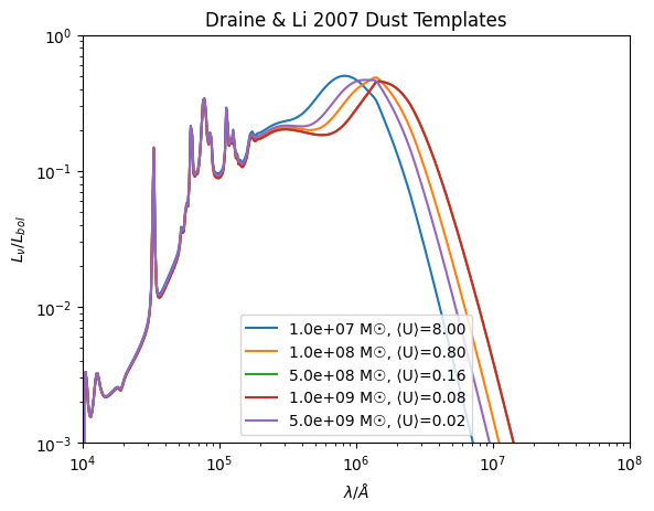
Draine & Li 2007 Dust Templates

The DrainLi07 generator implements the detailed dust emission templates from Draine & Li 2007. This is the most sophisticated dust model available, based on realistic dust grain physics and radiative transfer calculations.

Key features of the Draine & Li 2007 model:

• Physical dust model: Based on carbonaceous and silicate grain populations

• PAH emission: Includes polycyclic aromatic hydrocarbon features

• Radiation field parameters: Characterized by U_min, U_max, and gamma

• PAH fraction: Controlled by q_PAH parameter

• Dust mass scaling: Follows Magdis+2012 approach with L_dust/M_dust = 125

The model requires a pre-computed grid that can be downloaded using:

synthesizer-download --dust-grid

Grid Parameters

The DL07 grid is parameterized by:

• U_min: Minimum starlight intensity heating the majority of dust

• q_PAH: PAH mass fraction (0.47%, 1.12%, 1.77%, 4.58% for MW, LMC, SMC-like dust)

• gamma: Fraction of dust mass heated by starlight intensity > U_min

• alpha: Power-law index for U distribution (typically ≠ 1)

from synthesizer.grid import Grid

grid_name = "draine_li_dust_emission_grid_MW_3p1.hdf5"
grid = Grid(grid_name)
print("Grid axes:", grid.axes)
print("Grid shape:", grid.shape)

Grid axes: ['qpah', 'umin', 'alpha']
Grid shape: (11, 36, 1001)

for mdust in [1e7, 1e8, 5e8, 1e9, 5e9]:
    model = DraineLi07(
        grid,
        dust_mass=mdust * Msun,
        hydrogen_mass=1e10 * Msun,
        gamma=0.05,
        alpha=2.0,
    )
    sed = model.get_spectra(lam, ldust=1e10 * Lsun)

    # Normalise the SED to the bolometric luminosity
    sed._lnu /= sed._bolometric_luminosity

    # And plot...
    plt.loglog(
        sed.lam,
        sed.luminosity,
        label="{:.1e} M☉, ⟨U⟩={:.2f}".format(mdust, model.u_avg),
    )

plt.title("Draine & Li 2007 Dust Templates")
plt.xlabel(r"$ \lambda / \AA$")
plt.ylabel(r"$ L_{\nu} / L_{bol}$")
plt.xlim(1e4, 1e8)
plt.ylim(10**-3, 1)
plt.legend()
plt.show()