The Sed object
A Spectral Energy Distribution, or SED, describes the energy distribution of an emitting body as a function of frequency / wavelength. In Synthesizer, spectra are stored in Sed objects.
There are a number of different ways to generate spectra in Synthesizer, but in every case the resulting SED is always stored in an Sed object. An Sed object in Synthesizer is generally agnostic to where the input spectra has come from, as you’ll see below; they can therefore be initialised with any arbitrary wavelength and luminosity density arrays.
The Sed class contains a number of methods for calculating derived properties, such as broadband luminosities / fluxes (within wavelength windows or on filters) and spectral indices (e.g. balmer break, UV-continuum slope), and for modifying the spectra themselves, for example by applying an attenuation curve due to dust. Many of these methods are automatically used during emission generation with an EmissionModel, but they can also be used directly
from the Sed objects themselves.
In this section we cover the basics of instantiating and interacting with Sed objects, and how to use them to calculate derived properties.
[1]:
import matplotlib.pyplot as plt
import numpy as np
from unyt import Angstrom, Hz, erg, eV, s, um
Initialising an Sed object
Although Sed objects are generally generated by other classes, you can also create them directly. The simplest way to do this is to pass a wavelength array and a luminosity density array.
[2]:
from synthesizer import Sed

# Define some wavelengths and luminosities densities
lams = np.logspace(3, 5, 100) * Angstrom
lnus = np.logspace(26, 30, 100) * erg / (s * Hz)

# Create a Sed object
sed = Sed(lams, lnus)
Extracting a Sed from a Grid
We cover generating Sed objects from galaxies and their components in the Generating Emissions section of the emissions documentation. The simplest way to generate a real Sed object is to extract it from a Grid directly (see the Grids documentation for more details). First we need the Grid.
[3]:
from synthesizer.grid import Grid

# Load a SPS grid
grid = Grid("test_grid")
Now we have a grid, we can extract an Sed for a single grid point by stating the age and metallicity of the point we want to extract, converting that to the spectra’s index, and then extracting the spectra at that index.
Note that we multiply the spectra below by an “initial mass” of \(10^8 {M_\odot}\) because spectra in this Grid are in per unit initial mass, and we want the values for the rest of this section to make sense. This is mostly unimportant.
[4]:
log10age = 6.0  # log10(age/yr)
metallicity = 0.01
spectra_type = "incident"
grid_point = grid.get_grid_point(log10ages=log10age, metallicities=metallicity)
sed = grid.get_sed_at_grid_point(grid_point, spectra_type=spectra_type)
sed.lnu *= 1e8  # multiply initial stellar mass
Sed attributes
Like all objects in Synthesizer, printing a Sed object prints a tabular summary of the object.
[5]:
print(sed)
+----------------------------------------------------------------------------------------------------+
|                                                SED                                                 |
+---------------------------+------------------------------------------------------------------------+
| Attribute                 | Value                                                                  |
+---------------------------+------------------------------------------------------------------------+
| redshift                  | 0                                                                      |
+---------------------------+------------------------------------------------------------------------+
| ndim                      | 1                                                                      |
+---------------------------+------------------------------------------------------------------------+
| nlam                      | 9244                                                                   |
+---------------------------+------------------------------------------------------------------------+
| shape                     | (9244,)                                                                |
+---------------------------+------------------------------------------------------------------------+
| lam (9244,)               | 1.30e-04 Å -> 2.99e+11 Å (Mean: 9.73e+09 Å)                            |
+---------------------------+------------------------------------------------------------------------+
| nu (9244,)                | 1.00e+07 Hz -> 2.31e+22 Hz (Mean: 8.51e+19 Hz)                         |
+---------------------------+------------------------------------------------------------------------+
| lnu (9244,)               | 0.00e+00 erg/(Hz*s) -> 3.10e+29 erg/(Hz*s) (Mean: 9.16e+27 erg/(Hz*s)) |
+---------------------------+------------------------------------------------------------------------+
| bolometric_luminosity     | 7.014598446416371e+44 erg/s                                            |
+---------------------------+------------------------------------------------------------------------+
| energy (9244,)            | 4.14e-08 eV -> 9.56e+07 eV (Mean: 3.52e+05 eV)                         |
+---------------------------+------------------------------------------------------------------------+
| frequency (9244,)         | 1.00e+07 Hz -> 2.31e+22 Hz (Mean: 8.51e+19 Hz)                         |
+---------------------------+------------------------------------------------------------------------+
| llam (9244,)              | 0.00e+00 erg/(s*Å) -> 1.27e+42 erg/(s*Å) (Mean: 2.79e+40 erg/(s*Å))    |
+---------------------------+------------------------------------------------------------------------+
| luminosity (9244,)        | 0.00e+00 erg/s -> 9.95e+44 erg/s (Mean: 2.28e+43 erg/s)                |
+---------------------------+------------------------------------------------------------------------+
| luminosity_lambda (9244,) | 0.00e+00 erg/(s*Å) -> 1.27e+42 erg/(s*Å) (Mean: 2.79e+40 erg/(s*Å))    |
+---------------------------+------------------------------------------------------------------------+
| luminosity_nu (9244,)     | 0.00e+00 erg/(Hz*s) -> 3.10e+29 erg/(Hz*s) (Mean: 9.16e+27 erg/(Hz*s)) |
+---------------------------+------------------------------------------------------------------------+
| wavelength (9244,)        | 1.30e-04 Å -> 2.99e+11 Å (Mean: 9.73e+09 Å)                            |
+---------------------------+------------------------------------------------------------------------+
The most important attributes of a Sed are lam and lnu, the wavelengths and spectral luminosity density respectively.
[6]:
print(sed.lam)
print(sed.lnu)
[1.29662e-04 1.33601e-04 1.37660e-04 ... 2.97304e+11 2.98297e+11
 2.99293e+11] Å
[0. 0. 0. ... 0. 0. 0.] erg/(Hz*s)
These also have more descriptive aliases.
[7]:
print(sed.wavelength)
print(sed.luminosity_nu)
[1.29662e-04 1.33601e-04 1.37660e-04 ... 2.97304e+11 2.98297e+11
 2.99293e+11] Å
[0. 0. 0. ... 0. 0. 0.] erg/(Hz*s)
We can also get the luminosity (\(L\)) or spectral luminosity density per wavelength (\(L_{\lambda}\)).
[8]:
print(sed.luminosity)
print(sed.llam)
[0. 0. 0. ... 0. 0. 0.] erg/s
[0. 0. 0. ... 0. 0. 0.] erg/(s*Å)
Plotting a Sed
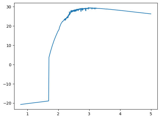
We could just take these attributes and plot them directly.
[9]:
plt.plot(np.log10(sed.lam), np.log10(sed.lnu))
plt.show()
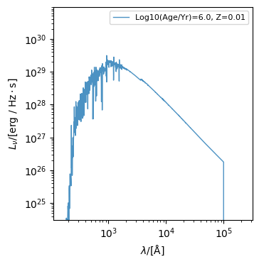
But Sed objects have their own bespoke plotting method, which is a little more sophisticated.
[10]:
fig, ax = sed.plot_spectra(label=f"log10(age/yr)={log10age}, Z={metallicity}")
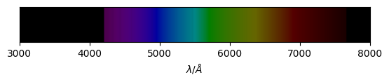
We can also visualise the spectrum as a rainbow.
[11]:
fig, ax = sed.plot_spectra_as_rainbow()
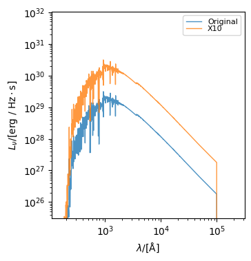
Arithmetic with Sed objects
Sed objects can be easily scaled via the * operator.
[12]:
sed_x_10 = sed * 10

fig, ax = sed.plot_spectra(label="original")
fig, ax = sed_x_10.plot_spectra(label="x10", fig=fig, ax=ax)
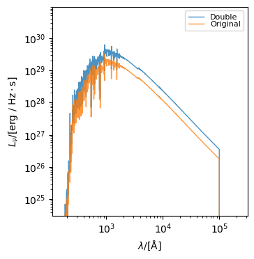
They can also be added and subtracted, which is useful for combining spectra.
[13]:
double_sed = sed + sed

fig, ax = double_sed.plot_spectra(label="double")
fig, ax = sed.plot_spectra(label="original", fig=fig, ax=ax)
Computing derived properties
There are numerous methods for computing derived properties from an Sed object. Here we will cover these methods.
Calculating the bolometric luminosity
We can calculate the bolometric luminosity of the Sed using the bolometric_luminosity property method.
[14]:
sed.bolometric_luminosity
[14]:
unyt_quantity(7.01459845e+44, 'erg/s')
This property integrates along the wavelength axis regardless of the shape of the Sed.
By default this will use a trapezoid integration method. To use the Simpson’s rule we can use the explicit measure_bolometric_luminosity method.
[15]:
sed.measure_bolometric_luminosity(integration_method="simps")
[15]:
unyt_quantity(6.99240325e+44, 'erg/s')
Computing luminosities in a window
You can also get the luminosity or lnu in a particular window by passing the wavelengths defining the limits of the window.
[16]:
sed.measure_window_luminosity((1400.0 * Angstrom, 1600.0 * Angstrom))
[16]:
unyt_quantity(4.04697126e+43, 'erg/s')
[17]:
sed.measure_window_lnu((1400.0 * Angstrom, 1600.0 * Angstrom))
[17]:
unyt_quantity(1.51388046e+29, 'erg/(Hz*s)')
Notice how units were provided with this window. These are required but also allow you to use an arbitrary unit system.
[18]:
sed.measure_window_luminosity((0.14 * um, 0.16 * um))
[18]:
unyt_quantity(4.04697126e+43, 'erg/s')
As for the bolometric luminosity, there are multiple integration methods that can be used for calculating the window. By default synthesizer will use the trapezoid method ("trapz"), but you can also take a simple average.
[19]:
sed.measure_window_lnu(
    (1400.0 * Angstrom, 1600.0 * Angstrom),
    integration_method="average",
)
[19]:
unyt_quantity(1.51387564e+29, 'erg/(Hz*s)')
Measuring breaks
You can also measure spectral breaks, such as the Balmer break, using the measure_break method and providing the wavelengths defining the limits of the break.
[20]:
sed.measure_break((3400, 3600) * Angstrom, (4150, 4250) * Angstrom)
[20]:
np.float64(0.8557102015137856)
For the Balmer break specifically, you can use the measure_balmer_break method, which will automatically use the correct wavelengths for the break.
[21]:
sed.measure_balmer_break()
[21]:
np.float64(0.8557102015137856)
Measuring line indices and spectral slopes
We can also measure absorption line indices, and spectral slopes (e.g. the UV spectral slope \(\beta\)).
Like the breaks we can measure an arbitrary line index by providing the wavelengths defining the limits of the windows used to measure the index.
[22]:
sed.measure_index(
    (1500, 1600) * Angstrom,
    (1400, 1500) * Angstrom,
    (1600, 1700) * Angstrom,
)
[22]:
unyt_quantity(5.80636059, 'Å')
Or we can use specialised methods like measure_d4000() or measure_beta() for the UV spectral slope.
[23]:
sed.measure_d4000()
[23]:
np.float64(0.9014948556841391)
[24]:
sed.measure_beta()
[24]:
np.float64(-2.9472024550639326)
By default this uses a single window and fits the spectrum by a power-law. However, we can also specify two windows as below, in which case the luminosity in each window is calculated and used to infer a slope.
[25]:
sed.measure_beta(window=(1250, 1750, 2250, 2750) * Angstrom)
[25]:
np.float64(-2.9532677904058)
Computing the ionising photon production rate
We can also measure ionising photon production rates at a particular ionisation energy.
[26]:
sed.calculate_ionising_photon_production_rate(
    ionisation_energy=13.6 * eV,
    limit=1000,
)
[26]:
unyt_quantity(9.81927283e+54, '1/s')
Observed frame SED
Everything up until now has been in the rest frame, with luminosity densities in units of erg/s/Hz or erg/s/Angstrom. A Sed object primarily stores the rest frame SED, and treats the observer frame SED as a derived property.
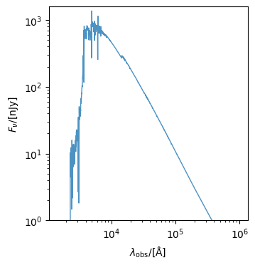
To move a Sed to the observer frame we simply call get_fnu with a cosmology, using an astropy.cosmology object, a redshift \(z\), and optionally an IGM absorption model (see here for details).
[27]:
from astropy.cosmology import Planck18 as cosmo

from synthesizer.emission_models.attenuation import Madau96

sed.get_fnu(cosmo, z=3.0, igm=Madau96)

fig, ax = sed.plot_observed_spectra(ylimits=(1, 10**3.2))
The result observer frame wavelenths and fluxes are stored in obslam and fnu respectively.
[28]:
print(sed)
+-------------------------------------------------------------------------------------------------------------------+
|                                                        SED                                                        |
+---------------------------+---------------------------------------------------------------------------------------+
| Attribute                 | Value                                                                                 |
+---------------------------+---------------------------------------------------------------------------------------+
| redshift                  | 3.00                                                                                  |
+---------------------------+---------------------------------------------------------------------------------------+
| ndim                      | 1                                                                                     |
+---------------------------+---------------------------------------------------------------------------------------+
| nlam                      | 9244                                                                                  |
+---------------------------+---------------------------------------------------------------------------------------+
| shape                     | (9244,)                                                                               |
+---------------------------+---------------------------------------------------------------------------------------+
| lam (9244,)               | 1.30e-04 Å -> 2.99e+11 Å (Mean: 9.73e+09 Å)                                           |
+---------------------------+---------------------------------------------------------------------------------------+
| nu (9244,)                | 1.00e+07 Hz -> 2.31e+22 Hz (Mean: 8.51e+19 Hz)                                        |
+---------------------------+---------------------------------------------------------------------------------------+
| lnu (9244,)               | 0.00e+00 erg/(Hz*s) -> 3.10e+29 erg/(Hz*s) (Mean: 9.16e+27 erg/(Hz*s))                |
+---------------------------+---------------------------------------------------------------------------------------+
| obslam (9244,)            | 5.19e-04 Å -> 1.20e+12 Å (Mean: 3.89e+10 Å)                                           |
+---------------------------+---------------------------------------------------------------------------------------+
| obsnu (9244,)             | 2.50e+06 Hz -> 5.78e+21 Hz (Mean: 2.13e+19 Hz)                                        |
+---------------------------+---------------------------------------------------------------------------------------+
| fnu (9244,)               | 0.00e+00 nJy -> 1.37e+03 nJy (Mean: 3.24e+01 nJy)                                     |
+---------------------------+---------------------------------------------------------------------------------------+
| bolometric_luminosity     | 7.014598446416371e+44 erg/s                                                           |
+---------------------------+---------------------------------------------------------------------------------------+
| energy (9244,)            | 4.14e-08 eV -> 9.56e+07 eV (Mean: 3.52e+05 eV)                                        |
+---------------------------+---------------------------------------------------------------------------------------+
| frequency (9244,)         | 1.00e+07 Hz -> 2.31e+22 Hz (Mean: 8.51e+19 Hz)                                        |
+---------------------------+---------------------------------------------------------------------------------------+
| llam (9244,)              | 0.00e+00 erg/(s*Å) -> 1.27e+42 erg/(s*Å) (Mean: 2.79e+40 erg/(s*Å))                   |
+---------------------------+---------------------------------------------------------------------------------------+
| luminosity (9244,)        | 0.00e+00 erg/s -> 9.95e+44 erg/s (Mean: 2.28e+43 erg/s)                               |
+---------------------------+---------------------------------------------------------------------------------------+
| luminosity_lambda (9244,) | 0.00e+00 erg/(s*Å) -> 1.27e+42 erg/(s*Å) (Mean: 2.79e+40 erg/(s*Å))                   |
+---------------------------+---------------------------------------------------------------------------------------+
| luminosity_nu (9244,)     | 0.00e+00 erg/(Hz*s) -> 3.10e+29 erg/(Hz*s) (Mean: 9.16e+27 erg/(Hz*s))                |
+---------------------------+---------------------------------------------------------------------------------------+
| wavelength (9244,)        | 1.30e-04 Å -> 2.99e+11 Å (Mean: 9.73e+09 Å)                                           |
+---------------------------+---------------------------------------------------------------------------------------+
| flam (9244,)              | 0.00e+00 erg/(cm**2*s*Å) -> 1.69e-18 erg/(cm**2*s*Å) (Mean: 2.38e-20 erg/(cm**2*s*Å)) |
+---------------------------+---------------------------------------------------------------------------------------+
| flux (9244,)              | 0.00e+00 Hz*nJy -> 8.25e+17 Hz*nJy (Mean: 1.36e+16 Hz*nJy)                            |
+---------------------------+---------------------------------------------------------------------------------------+
As you can see in the above print out, a number of other flux/observer frame attributes have now been added.
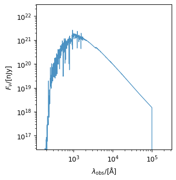
We can also derive the flux at a distance of 10 pc, using the get_fnu0 method. This is also the fallback used when get_fnu is called with a redshift of 0.
[29]:
sed.get_fnu0()

sed.plot_observed_spectra()
[29]:
(<Figure size 350x500 with 1 Axes>,
 <Axes: xlabel='$\\lambda_\\mathrm{obs}/[\\mathrm{\\AA}]$', ylabel='$F_{\\nu}/[\\mathrm{\\rm{nJy}}]$'>)
Photometry
If we want to derive photometry from a Sed object, we first need a FilterCollection or a photometric instrument carrying one. For more details on these see the Instruments and Filters documentation section of the documentation.
Now that we have the observer frame Sed we can use the get_photo_fnu method to calculate observed photometry. For rest frame photometry, we would instead use the get_photo_lnu method.
First lets get a JWST filter collection.
[30]:
from synthesizer.instruments import JWSTNIRCamWide

filters = JWSTNIRCamWide().filters
To get the photometry all we need to do is pass this filter set to the get_photo_fnu method.
[31]:
# Measure observed photometry
fluxes = sed.get_photo_fnu(filters)
print(fluxes)
-----------------------------------------------------
|                 PHOTOMETRY (FLUX)                 |
|------------------------------------|--------------|
| JWST/NIRCam.F070W (λ = 7.04e+03 Å) | 1.79e+20 nJy |
|------------------------------------|--------------|
| JWST/NIRCam.F090W (λ = 9.02e+03 Å) | 1.18e+20 nJy |
|------------------------------------|--------------|
| JWST/NIRCam.F115W (λ = 1.15e+04 Å) | 7.65e+19 nJy |
|------------------------------------|--------------|
| JWST/NIRCam.F150W (λ = 1.50e+04 Å) | 4.76e+19 nJy |
|------------------------------------|--------------|
| JWST/NIRCam.F200W (λ = 1.99e+04 Å) | 2.85e+19 nJy |
|------------------------------------|--------------|
| JWST/NIRCam.F277W (λ = 2.76e+04 Å) | 1.55e+19 nJy |
|------------------------------------|--------------|
| JWST/NIRCam.F356W (λ = 3.57e+04 Å) | 9.62e+18 nJy |
|------------------------------------|--------------|
| JWST/NIRCam.F444W (λ = 4.40e+04 Å) | 6.52e+18 nJy |
-----------------------------------------------------
This returns a PhotometryCollection object, for more details on these see the Photometry documentation.
Multidimensional SEDs
An Sed object can hold an arbitrarily shaped spectra array (as long as the final axis is the wavelength axis). One very common instance of this across Synthesizer is where you have spectra for particles making up a simulated galaxy. Below we will make a simple 2 particle example with 2 spectra.
[32]:
sed2 = Sed(sed.lam, np.array([sed.lnu, sed.lnu * 2]) * erg / s / Hz)
You can print an Sed object’s shape as if it were a numpy array.
[33]:
print(sed2.shape)
(2, 9244)
And all the methods we have seen so far will work on this multidimensional Sed object, as you’d expect.
[34]:
print(sed2.measure_window_lnu((1400, 1600) * Angstrom))
print(sed2.measure_beta())
print(sed2.measure_beta(window=(1250, 1750, 2250, 2750) * Angstrom))
print(sed2.measure_balmer_break())
print(
    sed2.measure_index(
        (1500, 1600) * Angstrom,
        (1400, 1500) * Angstrom,
        (1600, 1700) * Angstrom,
    )
)
print(
    sed2.calculate_ionising_photon_production_rate(
        ionisation_energy=13.6 * eV, limit=1000
    )
)
[1.51388046e+29 3.02776092e+29] erg/(Hz*s)
[-2.94720246 -2.94720246]
[-2.95326779 -2.95326779]
[0.8557102 0.8557102]
[5.80636059 5.80636059] Å
[9.81927283e+54 1.96385457e+55] 1/s
And even larger spectra. For example, here we convert an entire grid into a set of spectra and can compute properties just as if it were a single spectrum.
[35]:
sed3 = grid.get_sed(spectra_type="incident")
print(sed3.shape)

window = sed3.measure_window_lnu((1400, 1600) * Angstrom)

phot_rate = sed3.calculate_ionising_photon_production_rate(
    ionisation_energy=13.6 * eV, limit=1000
)
(51, 13, 9244)
Notice that the resulting shape has N-1 dimensions because we always act over the final wavelength axis.
[36]:
print(phot_rate.shape)
(51, 13)
Integrating Multidimensional SED objects
Multidimensional Sed objects can be integrated to produce a single spectrum by simply calling sum.
[37]:
print(sed3.shape)
int_sed3 = sed3.sum()
print(int_sed3.shape)
(51, 13, 9244)
(9244,)
Combining SEDs
Sed objects can be combined either via concatenation, to produce a single Sed holding multiple spectra, or by addition, to add the spectra contained in the input Sed objects (as shown above).
To concatenate spectra we use Sed.concat(). Sed.concat can take an arbitrary number of Sed objects to combine.
[38]:
print("Shapes before:", sed._lnu.shape, sed2._lnu.shape)
sed3 = sed2.concat(sed)
print("Combined shape:", sed3._lnu.shape)

sed4 = sed2.concat(sed, sed2, sed3)
print("Combined shape:", sed4._lnu.shape)
Shapes before: (9244,) (2, 9244)
Combined shape: (3, 9244)
Combined shape: (8, 9244)
Resampling SEDs
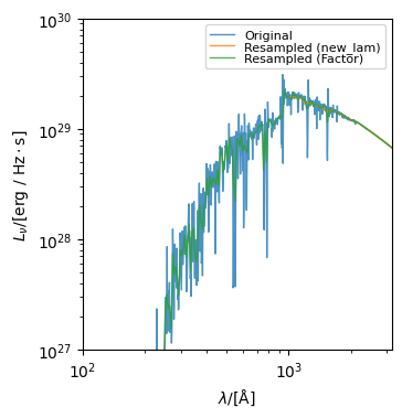
An Sed object can be resampled using the get_resampled_sed method which returns a new Sed object with the same spectra but resampled to a new wavelength array.
The resampling can either be done by downsampling by a factor, or by interpolation onto a new wavelength array.
[39]:
new_lam = np.logspace(3, 5, 100) * Angstrom
sed_factor_resampled = sed.get_resampled_sed(resample_factor=5)
sed_resampled = sed.get_resampled_sed(new_lam=new_lam)

fig, ax = sed.plot_spectra(label="Original")
fig, ax = sed_resampled.plot_spectra(
    label="Resampled (new_lam)", fig=fig, ax=ax
)
fig, ax = sed_factor_resampled.plot_spectra(
    label="Resampled (factor)",
    fig=fig,
    ax=ax,
    ylimits=(1e27, 1e30),
    xlimits=(10**2, 10**3.5),
)
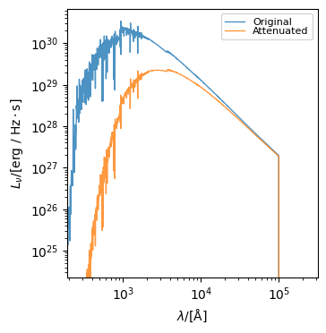
Applying attenuation
To apply attenuation to an Sed you can use the apply_attenuation method and pass the optical depth and a dust curve (see Attenuation for more details on dust curves).
[40]:
from synthesizer.emission_models.attenuation import PowerLaw

sed4_att = sed4.apply_attenuation(tau_v=0.7, dust_curve=PowerLaw(-1.0))

# Integrate the multidimensional spectra
int_sed4 = sed4.sum()
int_sed4_att = sed4_att.sum()

fig, ax = int_sed4.plot_spectra(label="Original")
fig, ax = int_sed4_att.plot_spectra(label="Attenuated", fig=fig, ax=ax)
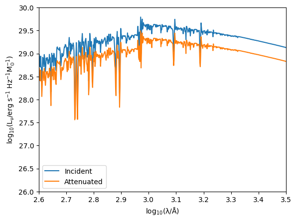
apply_attenuation can also accept a mask, which applies attenuation to specific spectra in a multidimensional Sed (like an Sed containing the spectra for multiple particles, for instance.)
[41]:
sed0_att = sed4.apply_attenuation(
    tau_v=0.7,
    dust_curve=PowerLaw(-1.0),
    mask=np.array([0, 1, 0, 0, 0, 0, 0, 0], dtype=bool),
)

plt.plot(np.log10(sed4.lam), np.log10(sed4.lnu[1, :]), label="Incident")
plt.plot(np.log10(sed4.lam), np.log10(sed0_att.lnu[0, :]), label="Attenuated")
plt.xlim(2.6, 3.5)
plt.ylim(26.0, 30.0)
plt.xlabel(r"$\rm log_{10}(\lambda/\AA)$")
plt.ylabel(r"$\rm log_{10}(L_{\nu}/erg\ s^{-1}\ Hz^{-1} M_{\odot}^{-1})$")
plt.legend()
plt.show()
plt.close()
Calculating transmission
If you have an attenuated SED, a natural quantity to calculate is the extinction of that spectra (\(A\)). This can be done either at the wavelengths of the Sed, an arbitrary wavelength/wavelength array, or at commonly used values (1500 and 5500 angstrom) using functions available in the emissions.sed submodule. Note that these functions return the extinction/attenuation in magnitudes. Below is a demonstration.
[42]:
from unyt import angstrom, um

from synthesizer.emissions import (
    get_attenuation,
    get_attenuation_at_1500,
    get_attenuation_at_5500,
    get_attenuation_at_lam,
)

# Get an intrinsic spectra
grid_point = grid.get_grid_point(log10ages=7, metallicities=0.01)
int_sed = grid.get_sed_at_grid_point(grid_point, spectra_type="incident")

# Apply an attenuation curve
att_sed = int_sed.apply_attenuation(tau_v=0.7, dust_curve=PowerLaw(-1.0))

# Get attenuation at sed.lam
attenuation = get_attenuation(int_sed, att_sed)

# Get attenuation at 5 microns
att_at_5 = get_attenuation_at_lam(5 * um, int_sed, att_sed)

# Get attenuation at an arbitrary range of wavelengths
att_at_range = get_attenuation_at_lam(
    np.linspace(5000, 10000, 5) * angstrom, int_sed, att_sed
)

# Get attenuation at 1500 angstrom
att_at_1500 = get_attenuation_at_1500(int_sed, att_sed)

# Get attenuation at 5500 angstrom
att_at_5500 = get_attenuation_at_5500(int_sed, att_sed)
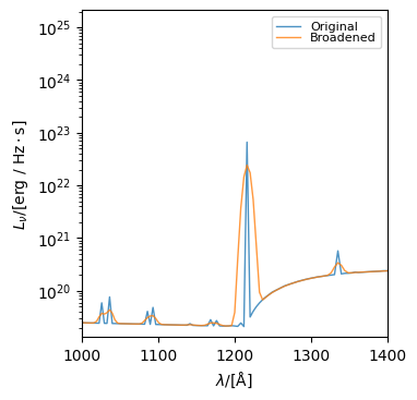
Doppler broadening
Sed objects also provide tools for producing Doppler-broadened versions of an SED. The method doppler_broaden returns a new SED broadened using a specified velocity dispersion. This can either operate in-place or return a new Sed object.
[43]:
from unyt import km, s

log10age = 6.0  # log10(age/yr)
metallicity = 0.01
spectra_type = "nebular"
grid_point = grid.get_grid_point(log10ages=log10age, metallicities=metallicity)

# Extract SED
sed = grid.get_sed_at_grid_point(grid_point, spectra_type=spectra_type)

# Apply Doppler broadening specifying a velocity
sed_broadened1 = sed.doppler_broaden(1000.0 * km / s)

# Plot to compare
fig, ax = sed.plot_spectra(label="original")
fig, ax = sed_broadened1.plot_spectra(
    label="broadened", fig=fig, ax=ax, xlimits=(1000, 1400)
)
ax.set_xscale("linear")
Thermal Broadening
There is also a variant of this method for thermal broadening, called thermally_broaden, which computes the broadening from a given temperature and mean molecular mass (which defaults to 1*amu). This can either operate in-place or return a new Sed object.
[44]:
from unyt import K

sed_thermal = sed.thermally_broaden(1e4 * K)
fig, ax = sed.plot_spectra(label="original")
fig, ax = sed_thermal.plot_spectra(
    label="thermally broadened", fig=fig, ax=ax, xlimits=(1000, 1400)
)
ax.set_xscale("linear")
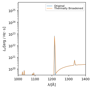
These methods are particularly useful when modelling environments where thermal motions contribute to line broadening, such as H II regions.
Note that, if you have a particle based component, self-consistent Doppler broadening based on particle velocities can be applied during emission generation by enabling vel_shift on an EmissionModel.