The Pipeline
If you have a galaxy catalog (either of Parametric origin or from a simulation), an `EmissionModel <../emission_models/emission_models.rst>`__, and a set of instruments you want observables for, you can easily write a pipeline to generate the observations you want using the Synthesizer UI. However, lets say you have a new catalog you want to run the same analysis on, or a whole different set of instruments you want to use. You could modify
your old pipeline or write a whole new pipeline, but thats a lot of work and boilerplate.
This is where the Pipeline shines. Instead, of having to write a pipeline, the Pipeline class is a high-level interface that allows you to easily generate observations for a given catalog, emission model, and set of instruments. All you need to do is set up the Pipeline object, attach the galaxies, and pass the instruments to the observable methods you want to generate with the necessary parameters. Possible observables include:
Spectra.
Emission Lines.
Photometry.
Images (with or without PSF convolution/noise).
Spectral data cubes (IFUs).
Spectroscopy on instrument-defined wavelength grids.
The Pipeline will generate all the requested observations for all (compatible) instruments and galaxies, before writing them out to a standardised HDF5 format.
As a bonus, the abstraction into the Pipeline class allows for easy parallelization of the analysis, not only over local threads but distributed over MPI.
The Pipeline workflow
When working with a Pipeline there are 4 distinct phases:
Instantiating the
Pipelineobject with the global properties and attaching galaxies.Signalling which observables to generate with which properties and instruments.
Running the
Pipeline.Writing the outputs.
We cover each of these phases in detail below.
Setting up a Pipeline object
Before we instatiate a pipeline we need to define its “dependencies”. These are an emission model, a set of instruments, and importantly some galaxies to “observe”.
Defining an emission model
The EmissionModel defines the emissions we’ll generate, including its origin and any reprocessing the emission undergoes. For more details see the EmissionModel docs.
For demonstration, we’ll use a simple premade IntrinsicEmission model which defines the intrinsic stellar emission (i.e. stellar emission without any ISM dust reprocessing).
[1]:
from synthesizer.emission_models import IntrinsicEmission
from synthesizer.grid import Grid

# Get the grid
grid_name = "test_grid"
grid = Grid(grid_name)

model = IntrinsicEmission(grid, fesc=0.1)
model.set_per_particle(True)  # we want per particle emissions
Defining the instruments
We don’t need any instruments if all we want is spectra at the spectral resolution of the Grid or emission lines. However, to get anything more sophisticated we need instrument objects that define the technical specifications of the observations we want to generate. In most workflows this means choosing the specialised class that matches the observing mode. For a full breakdown see the instrumentation docs.
Here we’ll define a simple set of specialised instruments including a subset of NIRCam filters carried by a PhotometricImager, a set of UVJ top hat filters carried by a PhotometricInstrument, a premade JWST MIRI instrument, and arbitrary SpectroscopicInstrument and IntegratedFieldUnit examples. We’ll then combine them in an InstrumentCollection and pass them explicitly to the observable methods below.
[2]:
import numpy as np
from unyt import angstrom, kpc

from synthesizer.instruments import (
    JWSTMIRI,
    UVJ,
    FilterCollection,
    IntegratedFieldUnit,
    PhotometricImager,
    PhotometricInstrument,
    SpectroscopicInstrument,
)

# Get the filters
lam = np.linspace(10**3, 10**5, 1000) * angstrom
webb_filters = FilterCollection(
    filter_codes=[
        f"JWST/NIRCam.{f}"
        for f in ["F090W", "F150W", "F200W", "F277W", "F356W", "F444W"]
    ],
    new_lam=lam,
)
uvj_filters = UVJ(new_lam=lam)

# Instantiate the specialised instruments
webb_inst = PhotometricImager(
    label="JWST.NIRCam",
    filters=webb_filters,
    resolution=1 * kpc,
)
miri_inst = JWSTMIRI()
uvj_inst = PhotometricInstrument(label="UVJ", filters=uvj_filters)
spectrometer = SpectroscopicInstrument(
    label="SpecInst", lam=np.logspace(3, 4, 100) * angstrom
)
ifu = IntegratedFieldUnit(
    label="IFU", lam=np.logspace(3, 4, 100) * angstrom, resolution=1 * kpc
)
instruments = webb_inst + miri_inst + uvj_inst + spectrometer + ifu

print(instruments)
+-------------------------------------------------------------------------------------------------+
|                                      INSTRUMENT COLLECTION                                      |
+-------------------+-----------------------------------------------------------------------------+
| Attribute         | Value                                                                       |
+-------------------+-----------------------------------------------------------------------------+
| all_filters       | <synthesizer.instruments.filters.FilterCollection object at 0x7f36400cc910> |
+-------------------+-----------------------------------------------------------------------------+
| ninstruments      | 5                                                                           |
+-------------------+-----------------------------------------------------------------------------+
| instrument_labels | [JWST.NIRCam, JWST.MIRI, UVJ, SpecInst, IFU,]                               |
+-------------------+-----------------------------------------------------------------------------+
| instruments       | JWST.NIRCam: PhotometricImager                                              |
|                   | JWST.MIRI: JWSTMIRI                                                         |
|                   | UVJ: PhotometricInstrument                                                  |
|                   | SpecInst: SpectroscopicInstrument                                           |
|                   | IFU: IntegratedFieldUnit                                                    |
+-------------------+-----------------------------------------------------------------------------+
Loading galaxies
You can load galaxies however you want but for this example we’ll load some CAMELS galaxies using the load_data module.
[3]:
from synthesizer import TEST_DATA_DIR
from synthesizer.load_data.load_camels import load_CAMELS_IllustrisTNG

# Create galaxy object
galaxies = load_CAMELS_IllustrisTNG(
    TEST_DATA_DIR,
    snap_name="camels_snap.hdf5",
    group_name="camels_subhalo.hdf5",
    physical=True,
)
Instantiating the Pipeline object
We have all the ingredients we need to instantiate a Pipeline object. All we need to do now is pass them into the Pipeline object alongside the number of threads we want to use during the analysis (in this notebook we’ll only use 1 for such a small handful of galaxies).
[4]:
from synthesizer.pipeline import Pipeline

pipeline = Pipeline(
    emission_model=model,
    nthreads=1,
    verbose=1,
)
                         ⠀⠀⠀⠀⠀⠀⠀⠀⠀⠀⢀⣀⣀⡀⠒⠒⠦⣄⡀⠀⠀⠀⠀⠀⠀⠀
                         ⠀⠀⠀⠀⠀⢀⣤⣶⡾⠿⠿⠿⠿⣿⣿⣶⣦⣄⠙⠷⣤⡀⠀⠀⠀⠀
                         ⠀⠀⠀⣠⡾⠛⠉⠀⠀⠀⠀⠀⠀⠀⠈⠙⠻⣿⣷⣄⠘⢿⡄⠀⠀⠀
                         ⠀⢀⡾⠋⠀⠀⠀⠀⠀⠀⠀⠀⠐⠂⠠⢄⡀⠈⢿⣿⣧⠈⢿⡄⠀⠀
                         ⢀⠏⠀⠀⠀⢀⠄⣀⣴⣾⠿⠛⠛⠛⠷⣦⡙⢦⠀⢻⣿⡆⠘⡇⠀⠀
                         ⠀⠀⠀+-+-+-+-+-+-+-+-+-+-+-+⡇⠀⠀
                         ⠀⠀⠀|S|Y|N|T|H|E|S|I|Z|E|R|⠃⠀⠀
                         ⠀⠀⢰+-+-+-+-+-+-+-+-+-+-+-+⠀⠀⠀
                         ⠀⠀⢸⡇⠸⣿⣷⠀⢳⡈⢿⣦⣀⣀⣀⣠⣴⣾⠟⠁⠀⠀⠀⠀⢀⡎
                         ⠀⠀⠘⣷⠀⢻⣿⣧⠀⠙⠢⠌⢉⣛⠛⠋⠉⠀⠀⠀⠀⠀⠀⣠⠎⠀
                         ⠀⠀⠀⠹⣧⡀⠻⣿⣷⣄⡀⠀⠀⠀⠀⠀⠀⠀⠀⠀⢀⣠⡾⠃⠀⠀
                         ⠀⠀⠀⠀⠈⠻⣤⡈⠻⢿⣿⣷⣦⣤⣤⣤⣤⣤⣴⡾⠛⠉⠀⠀⠀⠀
                         ⠀⠀⠀⠀⠀⠀⠈⠙⠶⢤⣈⣉⠛⠛⠛⠛⠋⠉⠀⠀⠀⠀⠀⠀⠀⠀
                         ⠀⠀⠀⠀⠀⠀⠀⠀⠀⠀⠀⠀⠉⠉⠉⠁⠀⠀⠀⠀⠀⠀⠀⠀⠀⠀


[00000.00]: Root emission model: intrinsic
[00000.00]: EmissionModel contains 10 individual models.
[00000.00]: EmissionModels split by emitter:
[00000.00]:    - galaxy:     0
[00000.00]:    - stellar:    10
[00000.00]:    - blackhole:  0
[00000.00]: EmissionModels split by operation type:
[00000.00]:    - extraction:   4
[00000.00]:    - combination:  3
[00000.00]:    - attenuating:  3
[00000.00]:    - generation:   0
Notice that we got a log out of the Pipeline object detailing the basic setup. The Pipeline will automatically output logging information to the console but this can be supressed by passing verbose=0 which limits the outputs to saying hello, goodbye, and any errors that occur.
Adding analysis functions
We could just run the analysis now and get whatever predefined outputs we want. However, we can also add our own analysis functions to the Pipeline object. These functions will be run on each galaxy in the catalog and can be used to generate any additional outputs we want. Importantly, these functions will be run after all other analysis has finished so they can make use of any outputs generated by the Pipeline object. They will also be run in the order they have been added allowing
access to anything derived in previous analysis functions.
Any extra analysis functions must obey the following rules:
It must calculate the “result” for a single galaxy at a time.
The function’s first argument must be the galaxy to calculate for.
It can take any number of additional arguments and keyword arguments.
It must either:
Return an array of values or a scalar, such that
np.array(<list of results>)is a valid operation. In other words, the results once combined for all galaxies should be an array of shape(n_galaxies, <result shape>).Return a dictionary where each result at the “leaves” of the dictionary structure is an array of values or a scalar, such that
np.array(<list of results>)is a valid operation. In other words, the dictionary of results once combined for all galaxies should be a dictionary with an array of shape(n_galaxies, <result shape>)at each “leaf”.
Below we’ll define an analysis function to compute stellar mass radii of each galaxy.
[5]:
def get_stellar_mass_radius(gal, fracs):
    """Compute the half mass radii.

    Args:
        gal (Galaxy):
            The galaxy to compute the half light radius of.
        fracs (list of float):
            The fractional radii to compute.
    """
    result = {}
    for frac in fracs:
        result[str(frac).replace(".", "p")] = gal.stars.get_attr_radius(
            "current_masses", frac
        )
    return result
To add this to the Pipeline we need to pass it along with a string defining the key under which the results will be stored in the HDF5 file and the fracs argument it requires.
[6]:
pipeline.add_analysis_func(
    get_stellar_mass_radius,
    result_key="Stars/HalfMassRadius",
    fracs=(0.2, 0.5, 0.8),
)
[00000.01]: Added analysis function: Stars/HalfMassRadius
This can also be done with simple lambda functions to include galaxy attributes in the output. For instance, the redshift.
[7]:
pipeline.add_analysis_func(lambda gal: gal.redshift, result_key="Redshift")
[00000.02]: Added analysis function: Redshift
Using the Pipeline Object
To run the analysis we need to instantiate the Pipeline, attach the galaxies, and then call the various observable generation methods to signal what observables (including any of the necessary arguments and/or instruments for each generation method) we want to generate. This approach allows you to explicitly control which observables you want to generate with a single line of code for each. Each of these getter methods signals to the Pipeline which observables you want to generate, with
what instruments and parameters, and eventually write out to the HDF5 file.
Attaching the galaxies
To include the galaxies we simply pass the list of Galaxy objects we defined above to the add_galaxies method. Note that this method is “destructive”, i.e. calling it multiple times will overwrite the galaxies previously attached.
[8]:
pipeline.add_galaxies(galaxies)
[00000.03]: Galaxies memory footprint: 0.45 MB
[00000.03]: Adding 10 galaxies took 3.797 ms.
Signalling the observables
Now we have the galaxies we can setup which observables we want. We do this by calling the various observable generation methods on the Pipeline object to signal which observables we want, followed by the run method to perform the analysis.
Spectra
We’ll start with the spectra.
[9]:
pipeline.get_spectra()
If we want fluxes, we can pass an astropy.cosmology object to the get_observed_fluxes method to get the fluxes in the observer frame.
[10]:
from astropy.cosmology import Planck18 as cosmo

pipeline.get_observed_spectra(cosmo)
Cosmic SED
The pipeline can also accumulate the total rest-frame and observer-frame cosmic SED across the attached galaxy sample. This can be done for the whole sample by simply calling get_cosmic_sed (or get_observed_cosmic_sed), or for a subsample selected based on integrated galaxy properties. This can be done for an arbitrary number of filters, and each can be given a label to distinguish them in the output file.
[11]:
pipeline.get_cosmic_sed()
pipeline.get_cosmic_sed(
    gal_attr="stellar_mass",
    lower_bound=1e8,
    upper_bound=1e9,
    label="LowStellarMass",
)
pipeline.get_observed_cosmic_sed(cosmo)
Line Emission
Next we’ll generate the emission lines. Here we can pass exactly which emission lines we want to generate based on line ID. We’ll just generate all lines offered by the Grid.
[12]:
pipeline.get_lines(line_ids=grid.available_lines)
Again, to get observed fluxes we can pass an astropy.cosmology object to the get_observed_lines method.
[13]:
pipeline.get_observed_lines(cosmo)
Photometry
Next, the photometry, where we need to pass the instruments defining the filters we want to apply and the label we want to apply that to. Unlike the previous methods that didn’t take instruments, these we can call multiple times with different instrument and label combinations to further control the generated observables.
Here we’ll generate intrinsic rest frame luminosities for the UVJ top hats, transmitted and intrinsic observed fluxes for the NIRCam filters and transmitted fluxes for UVJ top hat filters.
[14]:
pipeline.get_photometry_luminosities(uvj_inst, labels="intrinsic")
pipeline.get_photometry_fluxes(
    webb_inst, cosmo=cosmo, labels=["transmitted", "intrinsic"]
)
pipeline.get_photometry_fluxes(uvj_inst, cosmo=cosmo, labels="transmitted")
Imaging
Now, we’ll generate the images. Again, these are split into luminosity and flux flavours. Just like the photometry methods, we can call these multiple times with different instrument, label, and parameter combinations. These parameters include the field of view of the image, type of imaging (smoothed or histogram), and (if working in angular coordinates) a cosmology. If we are doing “smoothed” imaging (the default) where each particle is smoothed over its SPH kernel, we need to pass the kernel array, which we’ll extract here.
Note that had we defined instruments with PSFs and/or noise these would be applied automatically during the imaging process based on the instrument properties.
[15]:
from unyt import arcsecond

from synthesizer.kernel_functions import Kernel

# Get the SPH kernel
sph_kernel = Kernel()
kernel = sph_kernel.get_kernel()

pipeline.get_images_luminosity(
    webb_inst,
    fov=10 * kpc,
    kernel=kernel,
    labels="intrinsic",
)
pipeline.get_images_flux(
    webb_inst,
    fov=10 * kpc,
    kernel=kernel,
    labels=["transmitted", "intrinsic"],
)

pipeline.get_images_flux(
    miri_inst,
    fov=5.2 * arcsecond,
    kernel=kernel,
    cosmo=cosmo,
    labels="transmitted",
)
Spectroscopy (resolved/unresolved)
Similarly, we can generate both resolved and unresolved spectroscopy by passing the instruments and parameters, as well as the labels to act on (again for luminosity and flux flavours), to the data cube and spectroscopy methods. Though not demonstrated here, these methods can also be called multiple times with different configurations.
[16]:
# Get the resolved spectroscopy
pipeline.get_data_cubes_lnu(
    ifu,
    labels="intrinsic",
    kernel=kernel,
    fov=10 * kpc,
)
pipeline.get_data_cubes_fnu(
    ifu,
    labels="intrinsic",
    fov=5.2 * arcsecond,
    kernel=kernel,
    cosmo=cosmo,
)

# Get the unresolved spectroscopy
pipeline.get_spectroscopy_lnu(
    spectrometer,
    labels="intrinsic",
)
pipeline.get_spectroscopy_fnu(
    spectrometer,
    labels="intrinsic",
)
Running the Pipeline
Now we have every observable we want signalled for generation we can run the pipeline. This will generate all the observables on a galaxy by galaxy basis removing each galaxy from memory to reduce memory usage. This whole process will automatically be parallelized over the number of threads we defined when we instantiated the Pipeline object where available.
To run everything we simply call the run method.
[17]:
pipeline.run()
[00000.14]: Using 5 instruments.
[00000.14]: Instruments have 22 filters in total.
[00000.14]: Included instruments: UVJ, JWST.NIRCam, JWST.MIRI, IFU, SpecInst
[00000.14]: Instruments split by capability:
[00000.14]:    - photometry:             3
[00000.14]:    - spectroscopy:           2
[00000.14]:    - imaging:                2
[00000.14]:    - resolved spectroscopy:  1
[00000.18]: Pipeline memory footprint (MB): 528.4307727813721
[00000.18]: Running the pipeline...
[00000.18]: +------------+------------+------------+------------+------------+
[00000.18]: |    Galaxy #|      Nstars|        Ngas|         Nbh|      dt (s)|
[00000.18]: +------------+------------+------------+------------+------------+
[00000.77]: |           0|         278|          64|        None|        0.59|
[00002.04]: |           1|         656|           0|        None|        1.27|
[00002.93]: |           2|         441|          25|        None|        0.89|
[00004.28]: |           3|         726|           0|        None|        1.35|
[00004.40]: |           4|           8|         180|        None|        0.12|
[00004.54]: |           5|          26|           0|        None|        0.14|
[00005.59]: |           6|         569|           0|        None|        1.04|
[00005.97]: |           7|         165|           0|        None|        0.39|
[00006.33]: |           8|         149|           0|        None|        0.35|
[00007.26]: |           9|         461|           0|        None|        0.94|
[00007.26]: +------------+------------+------------+------------+------------+
[00007.26]: Computing 90 Lnu Spectra took 4.14 s
[00007.26]: Computing 90 Fnu Spectra took 544.41 ms
[00007.26]: Computing 10 Cosmic SED Lnu took 12.48 ms
[00007.26]: Computing 10 Cosmic SED Fnu took 7.19 ms
[00007.26]: Computing 60 Luminosities took 12.19 ms
[00007.27]: Computing 190 Fluxes took 48.21 ms
[00007.27]: Computing 22860 Emission Line Luminosities took 226.64 ms
[00007.27]: Computing 22860 Emission Line Fluxes took 84.88 ms
[00007.27]: Computing 60 Luminosity Images took 44.63 ms
[00007.27]: Computing 320 Flux Images took 389.09 ms
[00007.27]: Computing 100 Lnu Data Cubes took 370.32 ms
[00007.27]: Computing 100 Fnu Data Cubes took 375.88 ms
[00007.27]: Computing 10 Spectroscopy Lnu took 390.67 ms
[00007.27]: Computing 10 Spectroscopy Fnu took 381.77 ms
[00007.27]: Running 20 extra analyses took 7.25 ms
[00007.27]: Unpacking results took 13.32 ms
[00007.27]: Computing Stars/HalfMassRadius took 7.07 ms
[00007.27]: Computing Redshift took 0.10 ms
[00007.27]: Cleaning outputs took 3.969 ms.
Writing out the data
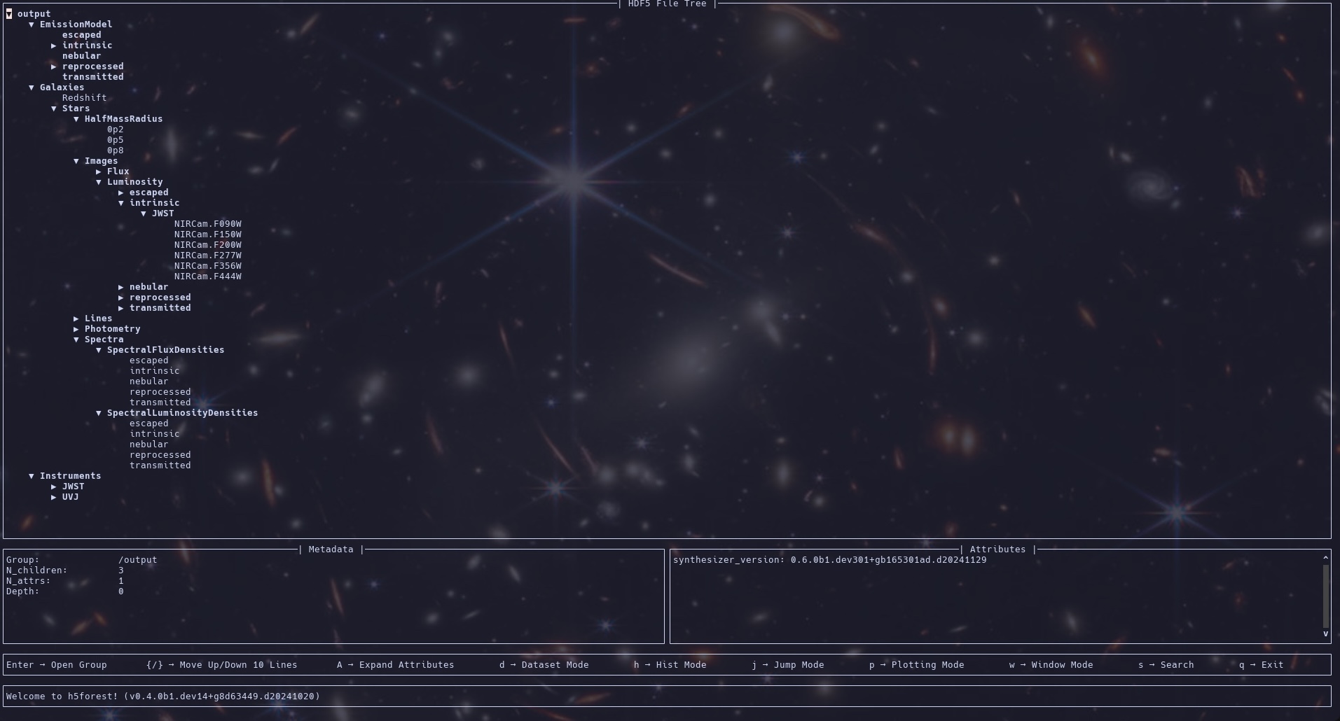
Finally, we write out the data to a HDF5 file. This file will contain all the observables we generated, as well as any additional analysis we ran. This file is structure to mirror the structure of Synthesizer objects, with each galaxy being a group, each component being a subgroup, and each individual observable being a dataset (or set of subgroups with the observables as datasets at their leaves in the case of a dicitonary attribute).
To write out the data we just pass the path to the file we want to write to to the write method.
Note that we all passing verbose=0 to silence the dataset timings for these docs. Otherwise, we would get timings for the writing of individual datasets. In the wild these timings are useful but here they’d just bloat the demo.
[18]:
pipeline.write("output.hdf5", verbose=0)
[00007.73]: Writing data took 449.398 ms.
[00007.73]: Total synthesis took 7.735 s.
[00007.73]: Goodbye!
Below is a view into the HDF5 file produced by the above pipeline (as shown by H5forest).
Timing the pipeline
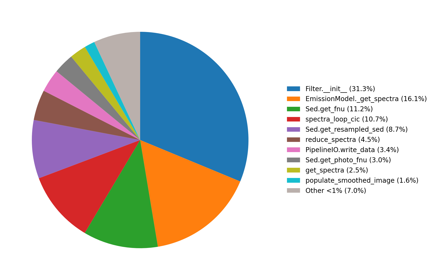
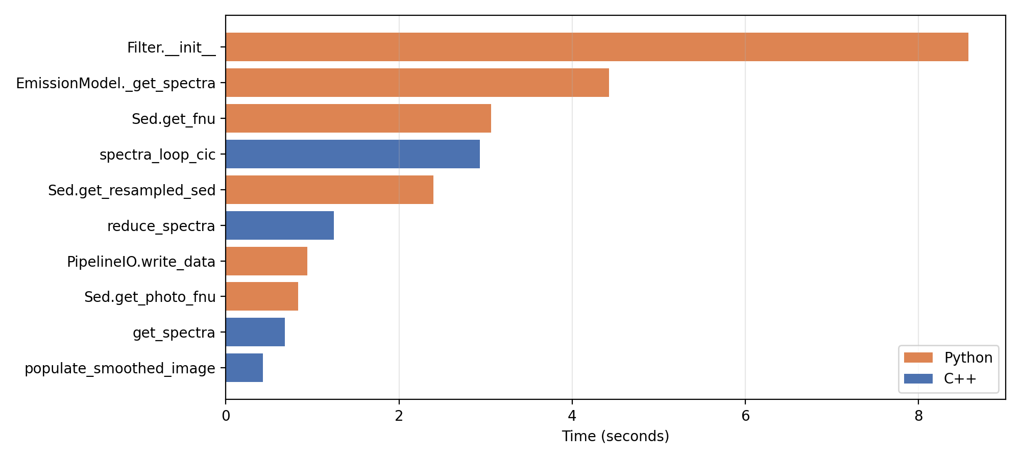
If Synthesizer has been installed with ATOMIC_TIMING enabled, the Pipeline can also produce a diagnostic timing report using analyse_timings. These timings are atomic and exclusive, meaning they only include the time spent in the explicitly timed blocks and account for any timers nested within other timers. More timers can be added by including tic and toc calls within the source code.
In the section below, we run the Pipeline and demonstrate what this looks like.
Putting it all together
Here is what the pipeline would look like without all the descriptive fluff…
[19]:
# Create galaxy object
galaxies = load_CAMELS_IllustrisTNG(
    TEST_DATA_DIR,
    snap_name="camels_snap.hdf5",
    group_name="camels_subhalo.hdf5",
    physical=True,
)

pipeline = Pipeline(model, report_memory=True)
pipeline.add_analysis_func(
    get_stellar_mass_radius,
    result_key="Stars/HalfMassRadius",
    fracs=(0.2, 0.5, 0.8),
)
pipeline.add_analysis_func(lambda gal: gal.redshift, result_key="Redshift")
pipeline.add_galaxies(galaxies)
pipeline.get_spectra()
pipeline.get_observed_spectra(cosmo)
pipeline.get_cosmic_sed()
pipeline.get_observed_cosmic_sed(cosmo)
pipeline.get_lines(line_ids=grid.available_lines)
pipeline.get_observed_lines(cosmo)
pipeline.get_photometry_luminosities(uvj_inst, webb_inst, miri_inst)
pipeline.get_photometry_fluxes(webb_inst)
pipeline.get_images_luminosity(
    webb_inst, fov=10 * kpc, kernel=kernel, labels="intrinsic"
)
pipeline.get_images_flux(
    webb_inst, fov=10 * kpc, kernel=kernel, labels="intrinsic"
)
pipeline.get_data_cubes_lnu(
    ifu, labels="intrinsic", kernel=kernel, fov=10 * kpc
)
pipeline.get_data_cubes_fnu(
    ifu, labels="intrinsic", kernel=kernel, fov=5.2 * arcsecond, cosmo=cosmo
)
pipeline.get_spectroscopy_lnu(spectrometer, labels="intrinsic")
pipeline.get_spectroscopy_fnu(spectrometer, labels="intrinsic")
pipeline.run()
pipeline.write("output.hdf5", verbose=0)
pipeline.analyse_timings("pipeline_timings")
⠀⠀⠀⠀⠀⠀⠀⠀⠀⠀⢀⣀⣀⡀⠒⠒⠦⣄⡀⠀⠀⠀⠀⠀⠀⠀
⠀⠀⠀⠀⠀⢀⣤⣶⡾⠿⠿⠿⠿⣿⣿⣶⣦⣄⠙⠷⣤⡀⠀⠀⠀⠀
⠀⠀⠀⣠⡾⠛⠉⠀⠀⠀⠀⠀⠀⠀⠈⠙⠻⣿⣷⣄⠘⢿⡄⠀⠀⠀
⠀⢀⡾⠋⠀⠀⠀⠀⠀⠀⠀⠀⠐⠂⠠⢄⡀⠈⢿⣿⣧⠈⢿⡄⠀⠀
⢀⠏⠀⠀⠀⢀⠄⣀⣴⣾⠿⠛⠛⠛⠷⣦⡙⢦⠀⢻⣿⡆⠘⡇⠀⠀
⠀⠀⠀+-+-+-+-+-+-+-+-+-+-+-+⡇⠀⠀
⠀⠀⠀|S|Y|N|T|H|E|S|I|Z|E|R|⠃⠀⠀
⠀⠀⢰+-+-+-+-+-+-+-+-+-+-+-+⠀⠀⠀
⠀⠀⢸⡇⠸⣿⣷⠀⢳⡈⢿⣦⣀⣀⣀⣠⣴⣾⠟⠁⠀⠀⠀⠀⢀⡎
⠀⠀⠘⣷⠀⢻⣿⣧⠀⠙⠢⠌⢉⣛⠛⠋⠉⠀⠀⠀⠀⠀⠀⣠⠎⠀
⠀⠀⠀⠹⣧⡀⠻⣿⣷⣄⡀⠀⠀⠀⠀⠀⠀⠀⠀⠀⢀⣠⡾⠃⠀⠀
⠀⠀⠀⠀⠈⠻⣤⡈⠻⢿⣿⣷⣦⣤⣤⣤⣤⣤⣴⡾⠛⠉⠀⠀⠀⠀
⠀⠀⠀⠀⠀⠀⠈⠙⠶⢤⣈⣉⠛⠛⠛⠛⠋⠉⠀⠀⠀⠀⠀⠀⠀⠀
⠀⠀⠀⠀⠀⠀⠀⠀⠀⠀⠀⠀⠉⠉⠉⠁⠀⠀⠀⠀⠀⠀⠀⠀⠀⠀
[00000.00]: Root emission model: intrinsic
[00000.00]: EmissionModel contains 10 individual models.
[00000.00]: EmissionModels split by emitter:
[00000.00]: - galaxy: 0
[00000.00]: - stellar: 10
[00000.00]: - blackhole: 0
[00000.00]: EmissionModels split by operation type:
[00000.00]: - extraction: 4
[00000.00]: - combination: 3
[00000.00]: - attenuating: 3
[00000.00]: - generation: 0
[00000.00]: Added analysis function: Stars/HalfMassRadius
[00000.00]: Added analysis function: Redshift
[00000.00]: Galaxies memory footprint: 0.45 MB
[00000.00]: Adding 10 galaxies took 2.324 ms.
[00000.03]: Using 5 instruments.
[00000.03]: Instruments have 22 filters in total.
[00000.03]: Included instruments: JWST.MIRI, UVJ, JWST.NIRCam, IFU, SpecInst
[00000.03]: Instruments split by capability:
[00000.03]: - photometry: 3
[00000.03]: - spectroscopy: 2
[00000.03]: - imaging: 2
[00000.03]: - resolved spectroscopy: 1
[00000.05]: Pipeline memory footprint (MB): 582.27099609375
[00000.05]: Running the pipeline...
[00000.05]: +------------+------------+------------+------------+------------+------------------------+------------------------+------------------------+
[00000.05]: | Galaxy #| Nstars| Ngas| Nbh| dt (s)| Memory footprint (MB)| Galaxy memory (MB)| Results memory (MB)|
[00000.05]: +------------+------------+------------+------------+------------+------------------------+------------------------+------------------------+
[00000.58]: | 0| 278| 64| None| 0.51| 589.74| 0.41| 1.44|
[00001.72]: | 1| 656| 0| None| 1.13| 591.05| 0.34| 2.82|
[00002.54]: | 2| 441| 25| None| 0.81| 592.38| 0.28| 4.21|
[00003.66]: | 3| 726| 0| None| 1.11| 593.69| 0.20| 5.59|
[00003.79]: | 4| 8| 180| None| 0.11| 595.06| 0.18| 6.99|
[00003.93]: | 5| 26| 0| None| 0.13| 596.44| 0.17| 8.37|
[00005.06]: | 6| 569| 0| None| 1.12| 597.76| 0.11| 9.76|
[00005.40]: | 7| 165| 0| None| 0.33| 599.12| 0.08| 11.14|
[00005.73]: | 8| 149| 0| None| 0.32| 600.50| 0.06| 12.55|
[00006.72]: | 9| 461| 0| None| 0.97| 601.83| 0.00| 13.93|
[00006.72]: +------------+------------+------------+------------+------------+------------------------+------------------------+------------------------+
[00006.72]: Computing 90 Lnu Spectra took 3.54 s
[00006.72]: Computing 90 Fnu Spectra took 468.45 ms
[00006.72]: Computing 10 Cosmic SED Lnu took 9.00 ms
[00006.72]: Computing 10 Cosmic SED Fnu took 7.29 ms
[00006.72]: Computing 1820 Luminosities took 98.99 ms
[00006.72]: Computing 540 Fluxes took 75.14 ms
[00006.72]: Computing 22860 Emission Line Luminosities took 224.29 ms
[00006.72]: Computing 22860 Emission Line Fluxes took 80.47 ms
[00006.72]: Computing 60 Luminosity Images took 44.69 ms
[00006.72]: Computing 60 Flux Images took 41.86 ms
[00006.72]: Computing 100 Lnu Data Cubes took 465.42 ms
[00006.72]: Computing 100 Fnu Data Cubes took 472.54 ms
[00006.72]: Computing 10 Spectroscopy Lnu took 477.48 ms
[00006.72]: Computing 10 Spectroscopy Fnu took 494.15 ms
[00006.72]: Running 20 extra analyses took 7.52 ms
[00006.72]: Unpacking results took 30.00 ms
[00006.72]: Computing Stars/HalfMassRadius took 7.31 ms
[00006.72]: Computing Redshift took 0.10 ms
[00006.73]: Cleaning outputs took 7.996 ms.
[00007.40]: Writing data took 670.361 ms.
[00007.40]: Total synthesis took 7.405 s.
[00007.40]: Goodbye!
[00007.40]: +-------------------------------------------------------+----------+--------------+-------+--------+
[00007.40]: | Operation | Time (s) | Fraction (%) | Count | Source |
[00007.40]: +-------------------------------------------------------+----------+--------------+-------+--------+
[00007.40]: | EmissionModel._get_spectra | 3.40 | 45.93 | 20 | Python |
[00007.40]: | Sed.get_resampled_sed | 3.21 | 43.39 | 120 | Python |
[00007.40]: | spectra_loop_cic | 2.49 | 33.68 | 240 | C |
[00007.40]: | reduce_spectra | 1.11 | 14.93 | 120 | C |
[00007.40]: | PipelineIO.write_data | 1.01 | 13.69 | 82 | Python |
[00007.40]: | compute_fnu | 0.84 | 11.37 | 360 | C |
[00007.40]: | get_spectra | 0.49 | 6.63 | 240 | C |
[00007.40]: | populate_smoothed_image | 0.42 | 5.65 | 100 | C |
[00007.40]: | Sed.get_fnu | 0.16 | 2.22 | 360 | Python |
[00007.40]: | LineCollection.get_flux | 0.16 | 2.21 | 360 | Python |
[00007.40]: | scale_spectra_2d | 0.16 | 2.16 | 180 | C |
[00007.40]: | EmissionModel._get_lines | 0.16 | 2.16 | 20 | Python |
[00007.40]: | FilterCollection.apply_filters | 0.12 | 1.67 | 560 | Python |
[00007.40]: | Pipeline._add_progress_row | 0.11 | 1.55 | 20 | Python |
[00007.40]: | Image.__init__ | 0.11 | 1.45 | 500 | Python |
[00007.40]: | Grid.__init__ | 0.10 | 1.31 | 1 | Python |
[00007.40]: | ParticleExtractor.generate_line | 0.08 | 1.10 | 80 | Python |
[00007.40]: | Sed.__init__ | 0.08 | 1.03 | 520 | Python |
[00007.40]: | compute_particle_seds.setup_output_arrays | 0.06 | 0.86 | 240 | C |
[00007.40]: | PhotometricInstrument.to_hdf5 | 0.06 | 0.77 | 6 | Python |
[00007.40]: | Filter._interpolate_wavelength | 0.05 | 0.73 | 138 | Python |
[00007.40]: | accepts(PhotometryCollection.__init__) | 0.05 | 0.65 | 560 | Python |
[00007.40]: | FilterCollection._get_batched_weights | 0.05 | 0.62 | 572 | Python |
[00007.40]: | Pipeline._unpack_results | 0.04 | 0.59 | 20 | Python |
[00007.40]: | PipelineIO.create_file_with_metadata | 0.04 | 0.58 | 2 | Python |
[00007.40]: | Pipeline.run.pop_chunk | 0.04 | 0.57 | 20 | Python |
[00007.40]: | accepts(ImagingBase.__init__) | 0.03 | 0.39 | 600 | Python |
[00007.40]: | Filter.__init__ | 0.03 | 0.34 | 22 | Python |
[00007.40]: | _generate_images_particle_smoothed.setup | 0.02 | 0.33 | 60 | Python |
[00007.40]: | accepts(Sed.__init__) | 0.02 | 0.33 | 520 | Python |
[00007.40]: | _generate_ifu_particle_smoothed.setup | 0.02 | 0.32 | 40 | Python |
[00007.40]: | ParticleExtractor.generate_lnu | 0.02 | 0.30 | 80 | Python |
[00007.40]: | PhotometricInstrument._comparison_state | 0.02 | 0.29 | 72 | Python |
[00007.40]: | Pipeline._get_cosmic_sed | 0.02 | 0.29 | 20 | Python |
[00007.40]: | _generate_images_particle_smoothed.unpack | 0.02 | 0.25 | 60 | Python |
[00007.40]: | _generate_image_collection_generic | 0.02 | 0.24 | 60 | Python |
[00007.40]: | IntegratedFieldUnit._generate_particle_component_cube | 0.02 | 0.24 | 40 | Python |
[00007.40]: | get_particle_indices_and_fracs | 0.02 | 0.23 | 240 | C |
[00007.40]: | ImageCollection.__init__ | 0.02 | 0.23 | 60 | Python |
[00007.40]: | Pipeline.run.print_progress_header | 0.02 | 0.22 | 2 | Python |
[00007.40]: | Pipeline._get_observed_cosmic_sed | 0.01 | 0.20 | 20 | Python |
[00007.40]: | Pipeline._run_extra_analysis.Stars/HalfMassRadius | 0.01 | 0.19 | 20 | Python |
[00007.40]: | Pipeline._clean_outputs | 0.01 | 0.16 | 2 | Python |
[00007.40]: | FilterCollection.resample_filters | 0.01 | 0.15 | 12 | Python |
[00007.40]: | Kernel.get_kernel | 0.01 | 0.15 | 1 | Python |
[00007.40]: | SpectralCube.__init__ | 0.01 | 0.15 | 40 | Python |
[00007.40]: | accepts(LineCollection.__init__) | 9.96e-03 | 0.13 | 400 | Python |
[00007.40]: | Extractor.__init__ | 9.95e-03 | 0.13 | 160 | Python |
[00007.40]: | Extractor.get_emitter_attrs | 9.76e-03 | 0.13 | 160 | Python |
[00007.40]: | Filter._get_weighted_integration_data | 9.64e-03 | 0.13 | 132 | Python |
[00007.40]: | PhotometryCollection.__init__ | 9.22e-03 | 0.12 | 560 | Python |
[00007.40]: | Pipeline.run | 7.71e-03 | 0.10 | 2 | Python |
[00007.40]: | Sed.scale | 6.97e-03 | 0.09 | 60 | Python |
[00007.40]: | Pipeline._get_observed_spectra | 6.26e-03 | 0.08 | 20 | Python |
[00007.40]: | Pipeline.add_galaxies | 6.18e-03 | 0.08 | 2 | Python |
[00007.40]: | Filter.prepare_for_grid | 5.58e-03 | 0.08 | 44 | Python |
[00007.40]: | Sed.get_photo_fnu | 5.23e-03 | 0.07 | 320 | Python |
[00007.40]: | ParticleStars.__init__ | 5.20e-03 | 0.07 | 20 | Python |
[00007.40]: | LineCollection.__init__ | 4.73e-03 | 0.06 | 400 | Python |
[00007.40]: | Sed.get_photo_lnu | 3.73e-03 | 0.05 | 240 | Python |
[00007.40]: | Pipeline._get_spectra | 3.65e-03 | 0.05 | 20 | Python |
[00007.40]: | accepts(Stars.__init__) | 3.57e-03 | 0.05 | 20 | Python |
[00007.40]: | _generate_images_particle_smoothed | 3.55e-03 | 0.05 | 60 | Python |
[00007.40]: | accepts(Particles.__init__) | 3.41e-03 | 0.05 | 40 | Python |
[00007.40]: | ModelQueue.__init__.compile | 3.40e-03 | 0.05 | 40 | Python |
[00007.40]: | Galaxy.get_data_cube | 3.17e-03 | 0.04 | 40 | Python |
[00007.40]: | _generate_ifu_particle_smoothed | 3.15e-03 | 0.04 | 40 | Python |
[00007.40]: | LineCollection.scale | 2.90e-03 | 0.04 | 60 | Python |
[00007.40]: | Pipeline._get_images_flux | 2.79e-03 | 0.04 | 20 | Python |
[00007.40]: | accepts(Galaxy.load_stars) | 2.52e-03 | 0.03 | 20 | Python |
[00007.40]: | Gas.__init__ | 2.45e-03 | 0.03 | 20 | Python |
[00007.40]: | Pipeline._get_images_luminosity | 2.41e-03 | 0.03 | 20 | Python |
[00007.40]: | ModelQueue.__init__.collect_tree | 2.39e-03 | 0.03 | 40 | Python |
[00007.40]: | PhotometricImager.to_hdf5 | 2.26e-03 | 0.03 | 4 | Python |
[00007.40]: | accepts(Gas.__init__) | 2.07e-03 | 0.03 | 20 | Python |
[00007.40]: | SpectroscopicInstrument.to_hdf5 | 2.04e-03 | 0.03 | 4 | Python |
[00007.40]: | accepts(Filter._interpolate_wavelength) | 1.98e-03 | 0.03 | 138 | Python |
[00007.40]: | Pipeline._get_photometry_fluxes | 1.95e-03 | 0.03 | 20 | Python |
[00007.40]: | accepts(Galaxy.load_gas) | 1.93e-03 | 0.03 | 20 | Python |
[00007.40]: | Pipeline._get_observed_lines | 1.74e-03 | 0.02 | 20 | Python |
[00007.40]: | Pipeline._get_photometry_luminosities | 1.72e-03 | 0.02 | 20 | Python |
[00007.40]: | Pipeline._get_spectroscopy_lnu | 1.61e-03 | 0.02 | 20 | Python |
[00007.40]: | weight_loop_cic | 1.60e-03 | 0.02 | 20 | C |
[00007.40]: | Pipeline._get_spectroscopy_fnu | 1.55e-03 | 0.02 | 20 | Python |
[00007.40]: | SpectroscopicInstrument.apply_lam_array | 1.55e-03 | 0.02 | 80 | Python |
[00007.40]: | compute_particle_seds | 1.44e-03 | 0.02 | 240 | C |
[00007.40]: | construct_cell_tree | 1.41e-03 | 0.02 | 100 | C |
[00007.40]: | Pipeline._get_lines | 1.22e-03 | 0.02 | 20 | Python |
[00007.40]: | FilterCollection.__init__ | 1.18e-03 | 0.02 | 3 | Python |
[00007.40]: | IntegratedFieldUnit.to_hdf5 | 1.07e-03 | 0.01 | 2 | Python |
[00007.40]: | EmissionModel.__init__ | 1.04e-03 | 0.01 | 10 | Python |
[00007.40]: | compute_integrated_sed | 1.02e-03 | 0.01 | 240 | C |
[00007.40]: | accepts(SpectralCube.__init__) | 8.96e-04 | 0.01 | 40 | Python |
[00007.40]: | IntegratedFieldUnit.generate_data_cube | 8.91e-04 | 0.01 | 40 | Python |
[00007.40]: | PhotometricImager._comparison_state | 8.58e-04 | 0.01 | 48 | Python |
[00007.40]: | Pipeline._get_data_cubes_fnu | 8.29e-04 | 0.01 | 20 | Python |
[00007.40]: | Pipeline.__init__ | 8.19e-04 | 0.01 | 2 | Python |
[00007.40]: | Pipeline._get_data_cubes_lnu | 7.59e-04 | 0.01 | 20 | Python |
[00007.40]: | Overhead | 0.00 | 0.00 | - | N/A |
[00007.40]: | Total | 7.41 | 100.00 | - | N/A |
[00007.40]: +-------------------------------------------------------+----------+--------------+-------+--------+
Note here that we set report_memory=True when we instantiated the Pipeline. This caused the pipeline to probe the memory usage after each galaxy is processed and report it. While this is extremely useful information for debugging purposes, it is also extremely expensive to calculate and is thus turned off by default.
Below are the timing plots produced by the analyse_timings method.
Running a subset of observables
If you only want to generate a subset of observables then its as simple as only calling the methods for those observables. However, some observables are dependent on others.
For instance, to generate observed fluxes you need to have already generated observer frame spectra. If you signal you want one of these “downstream” observables without signalling the “upstream” observable then the Pipeline will automatically generate the upstream observable for you but they will not be written out to the HDF5 file.
The only difference is that you must supply the method you are calling with the arguments required to generate the upstream observable. Don’t worry though, the Pipeline will automatically tell you what is missing if you forget something.
We demonstrate this below by only selecting only the observed fluxes and observed emission lines.
[20]:
# Create galaxy object
galaxies = load_CAMELS_IllustrisTNG(
    TEST_DATA_DIR,
    snap_name="camels_snap.hdf5",
    group_name="camels_subhalo.hdf5",
    physical=True,
)
# Set up the pipeline
pipeline = Pipeline(model)
pipeline.add_galaxies(galaxies)
pipeline.get_observed_lines(cosmo, line_ids=grid.available_lines)
pipeline.get_photometry_fluxes(webb_inst, cosmo=cosmo)
                         ⠀⠀⠀⠀⠀⠀⠀⠀⠀⠀⢀⣀⣀⡀⠒⠒⠦⣄⡀⠀⠀⠀⠀⠀⠀⠀
                         ⠀⠀⠀⠀⠀⢀⣤⣶⡾⠿⠿⠿⠿⣿⣿⣶⣦⣄⠙⠷⣤⡀⠀⠀⠀⠀
                         ⠀⠀⠀⣠⡾⠛⠉⠀⠀⠀⠀⠀⠀⠀⠈⠙⠻⣿⣷⣄⠘⢿⡄⠀⠀⠀
                         ⠀⢀⡾⠋⠀⠀⠀⠀⠀⠀⠀⠀⠐⠂⠠⢄⡀⠈⢿⣿⣧⠈⢿⡄⠀⠀
                         ⢀⠏⠀⠀⠀⢀⠄⣀⣴⣾⠿⠛⠛⠛⠷⣦⡙⢦⠀⢻⣿⡆⠘⡇⠀⠀
                         ⠀⠀⠀+-+-+-+-+-+-+-+-+-+-+-+⡇⠀⠀
                         ⠀⠀⠀|S|Y|N|T|H|E|S|I|Z|E|R|⠃⠀⠀
                         ⠀⠀⢰+-+-+-+-+-+-+-+-+-+-+-+⠀⠀⠀
                         ⠀⠀⢸⡇⠸⣿⣷⠀⢳⡈⢿⣦⣀⣀⣀⣠⣴⣾⠟⠁⠀⠀⠀⠀⢀⡎
                         ⠀⠀⠘⣷⠀⢻⣿⣧⠀⠙⠢⠌⢉⣛⠛⠋⠉⠀⠀⠀⠀⠀⠀⣠⠎⠀
                         ⠀⠀⠀⠹⣧⡀⠻⣿⣷⣄⡀⠀⠀⠀⠀⠀⠀⠀⠀⠀⢀⣠⡾⠃⠀⠀
                         ⠀⠀⠀⠀⠈⠻⣤⡈⠻⢿⣿⣷⣦⣤⣤⣤⣤⣤⣴⡾⠛⠉⠀⠀⠀⠀
                         ⠀⠀⠀⠀⠀⠀⠈⠙⠶⢤⣈⣉⠛⠛⠛⠛⠋⠉⠀⠀⠀⠀⠀⠀⠀⠀
                         ⠀⠀⠀⠀⠀⠀⠀⠀⠀⠀⠀⠀⠉⠉⠉⠁⠀⠀⠀⠀⠀⠀⠀⠀⠀⠀


[00000.00]: Root emission model: intrinsic
[00000.00]: EmissionModel contains 10 individual models.
[00000.00]: EmissionModels split by emitter:
[00000.00]:    - galaxy:     0
[00000.00]:    - stellar:    10
[00000.00]:    - blackhole:  0
[00000.00]: EmissionModels split by operation type:
[00000.00]:    - extraction:   4
[00000.00]:    - combination:  3
[00000.00]:    - attenuating:  3
[00000.00]:    - generation:   0
[00000.00]: Galaxies memory footprint: 0.45 MB
[00000.00]: Adding 10 galaxies took 1.385 ms.
If we want to see which observables we have signalled for generation we can call the report_operations method, which will print out a list of all observables we have signalled for generation and whether they will be written out to the HDF5 file.
[21]:
pipeline.report_operations()
[00000.01]: ------------------------------------------------------------
[00000.01]:                                      Compute?         Write?
[00000.01]: Line of Sight Optical Depths            False            N/A
[00000.01]: SFZH                                    False          False
[00000.01]: SFH                                     False          False
[00000.01]: Lnu Spectra                              True          False
[00000.01]: Fnu Spectra                              True          False
[00000.01]: Cosmic SED Lnu                          False          False
[00000.01]: Cosmic SED Fnu                          False          False
[00000.01]: Photometric Luminosities                False          False
[00000.01]: Photometric Fluxes                       True           True
[00000.01]: Emission Line Luminosities               True          False
[00000.01]: Emission Line Fluxes                     True           True
[00000.01]: Luminosity Images                       False          False
[00000.01]: Flux Images                             False          False
[00000.01]: Lnu Data Cubes                          False          False
[00000.01]: Fnu Data Cubes                          False          False
[00000.01]: Spectroscopy Lnu                        False          False
[00000.01]: Spectroscopy Fnu                        False          False
[00000.01]: ------------------------------------------------------------
Note here we have can see all the possible operations we could have signalled for generation but only the observed fluxes and observed emission lines will be written out to the HDF5 file since these are the getters we called.
Hybrid parallelism with MPI
Above we demonstrated how to run a pipeline using only local shared memory parallelism. We can also use mpi4py to not only use the shared memory parallelism but also distribute the analysis across multiple nodes (hence “hybrid parallelism”).
Instatiating a Pipeline when using MPI
To make use of MPI we only need to make a couple changes to running the pipeline. The first is simply that we need to pass the comm object to the Pipeline object when we instantiate it.
from mpi4py import MPI

pipeline = Pipeline(
    gal_loader_func=galaxy_loader,
    emission_model=model,
    n_galaxies=10,
    instruments=instruments,
    nthreads=4,
    verbose=1,
    comm=MPI.COMM_WORLD,
)
Here verbose=1 will mean only rank 0 will output logging information. If you want all ranks to output logging information you should set verbose=2. verbose=0 will silence all outputs apart from the greeting, total timing and errors as before.
Adding galaxies with MPI
We also need to partition the galaxies before we attach them to a Pipeline. For now we provide no mechanisms for this, it is entirely up to you how to split galaxies across the ranks. The important thing is that you only pass the galaxies on a rank to add_galaxies.
Writing out results with MPI
When running a distributed Pipeline you have several options for writing out the data. Regardless of which approach is used the process to write the outputs is the same as the shared memory version shown above (i.e. we call the write method). We detail each of these below.
Collective I/O [WIP]
If you have installed h5py with parallel HDF5 its possible to write collectively to a single HDF5 file. A Pipeline will detect if parallel h5py is available and will automatically chose this option if possible.
Individual I/O
When collective I/O operations aren’t available we produce a file per MPI rank. This is the most efficient method since communicating the results to a single rank for outputting is not only extremely time consuming but can also lead to communication errors when the outputs are sufficiently large.
Once the rank files have been written out we provide 2 options for combining them into a single file, note that working with the rank files is entirely possible though.
Combination into a single physical file: calling
combine_fileswill copy all the data across from each rank file into a single file before deleting each individual rank file. This is clean with regard to what is left, but is extremely time consuming.Combination into a single virtual file: calling
combine_files_virtualwill make a single file with symlinks to all the rank data in virtual datasets. This is far more efficient and gives the same interaction behaviour as the copy option (i.e. a single file to interact with) but does mean all the rank files must be kept alongside the virtual file.
Memory-aware chunking
If your catalogue contains a large spread in galaxy sizes, the biggest particle galaxies can dominate the transient memory usage of the Pipeline and in the worst cases lead to out of memory errors. This is most noticeable when temporary per-particle spectra using large per-particle EmissionModels that can contain numerous interim per-particle spectra.
In this situation you can pass max_npart when constructing the Pipeline. This will split large galaxies into smaller stellar chunks, process those chunks sequentially, and accumulate the pipeline outputs back onto the parent galaxy without holding on to dangerous memory footprints in the process.
This is most useful when there is a large imbalance between the biggest and smallest galaxies in the sample and memory, rather than runtime, is the main concern.
pipeline = Pipeline(
    emission_model=model,
    nthreads=4,
    max_npart=10000,
)