Spatial-resampling attribute modes

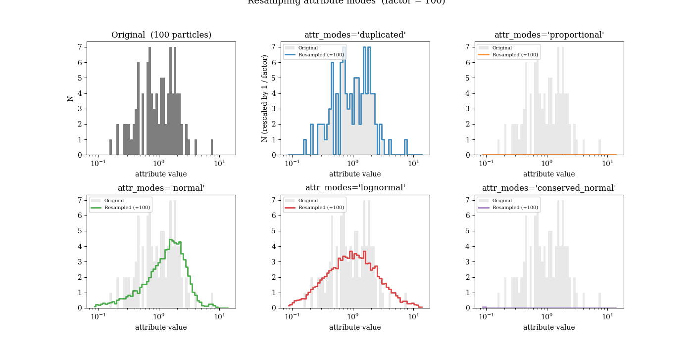
Demonstrates the five resample_by_mode() modes available via the attr_modes keyword of spatially_resample() (and the Stars equivalent).

A toy gas population of 100 particles carries a single extra attribute (my_attribute) with a well-defined lognormal initial distribution. Each particle is split into 100 children (factor = 100), yielding 10 000 resampled particles. Histograms show how each mode transforms the distribution — the resampled count in each bin is divided by the factor so the histogram heights are directly comparable to the original.

Modes

"duplicated" (default)

Every child inherits the parent value unchanged. The histogram is a scaled copy of the original.

"proportional"

Each child receives value / factor, conserving the total sum. The distribution shifts left by a factor of 100.

"normal"

Children are drawn from Normal(value, σ) where σ defaults to the population standard deviation. Histograms broaden around each parent.

"lognormal"

Like "normal" but in log-space; best for positive-definite quantities (metallicity, SFR, ages).

"conserved_normal"

Starts from the proportional split, adds Gaussian scatter, then renormalises each group so the children sum exactly to the parent value. Scatter with exact conservation.

import matplotlib.pyplot as plt
import numpy as np
from unyt import Mpc, Msun, km, s

from synthesizer.kernel_functions import Kernel
from synthesizer.particle.gas import Gas

plt.rcParams["font.family"] = "DeJavu Serif"
plt.rcParams["font.serif"] = ["Times New Roman"]

# ---------------------------------------------------------------------------
# Toy data: 100 gas particles with a lognormal synthetic attribute
# ---------------------------------------------------------------------------
NP = 100
FACTOR = 100
rng = np.random.default_rng(42)

# Lognormal attribute — reasonable prototype for metallicity, SFR, dust, etc.
attribute = 10 ** rng.normal(0.0, 0.4, NP)

gas = Gas(
    masses=rng.uniform(0.5e6, 2e6, NP) * Msun,
    metallicities=rng.uniform(0.005, 0.025, NP),
    coordinates=rng.uniform(-1, 1, (NP, 3)) * Mpc,
    velocities=rng.uniform(-50, 50, (NP, 3)) * (km / s),
    smoothing_lengths=np.ones(NP) * 0.3 * Mpc,
    redshift=0.1,
    my_attribute=attribute,
)

# ---------------------------------------------------------------------------
# Resample under each mode
# ---------------------------------------------------------------------------
g_dup = gas.spatially_resample(FACTOR, seed=1, kernel=Kernel("cubic"))
g_prop = gas.spatially_resample(
    FACTOR,
    seed=1,
    kernel=Kernel("cubic"),
    attr_modes={"my_attribute": "proportional"},
)
g_norm = gas.spatially_resample(
    FACTOR,
    seed=1,
    kernel=Kernel("cubic"),
    attr_modes={"my_attribute": "normal"},
)
g_logn = gas.spatially_resample(
    FACTOR,
    seed=1,
    kernel=Kernel("cubic"),
    attr_modes={"my_attribute": "lognormal"},
)
g_cons = gas.spatially_resample(
    FACTOR,
    seed=1,
    kernel=Kernel("cubic"),
    attr_modes={"my_attribute": "conserved_normal"},
)

# ---------------------------------------------------------------------------
# Plot
# ---------------------------------------------------------------------------
bins = np.logspace(
    np.log10(attribute.min() * 0.5), np.log10(attribute.max() * 2), 60
)

modes = [
    ("duplicated", g_dup.my_attribute, "tab:blue"),
    ("proportional", g_prop.my_attribute, "tab:orange"),
    ("normal", g_norm.my_attribute, "tab:green"),
    ("lognormal", g_logn.my_attribute, "tab:red"),
    ("conserved_normal", g_cons.my_attribute, "tab:purple"),
]

fig, axes = plt.subplots(
    2, 3, figsize=(14, 7), gridspec_kw=dict(wspace=0.3, hspace=0.35)
)
axes = axes.flatten()

# Panel 0: original distribution
ax = axes[0]
ax.hist(attribute, bins=bins, color="0.4", alpha=0.85)
ax.set_xscale("log")
ax.set_xlabel("attribute value")
ax.set_ylabel("N")
ax.set_title(f"Original  ({NP} particles)")

# Panels 1–5: each mode overlaid on the original
for i, (name, vals, colour) in enumerate(modes):
    ax = axes[i + 1]
    # Original histogram (background)
    ax.hist(attribute, bins=bins, color="0.7", alpha=0.3, label="Original")
    # Resampled histogram, scaled down by the factor so peak heights
    # are directly comparable to the original.
    counts, bin_edges = np.histogram(vals, bins=bins)
    bin_centres = np.sqrt(bin_edges[1:] * bin_edges[:-1])
    ax.step(
        bin_centres,
        counts / FACTOR,
        where="mid",
        color=colour,
        lw=2,
        alpha=0.85,
        label=f"Resampled (÷{FACTOR})",
    )
    ax.set_xscale("log")
    ax.set_xlabel("attribute value")
    if i == 0:
        ax.set_ylabel("N (rescaled by 1 / factor)")
    ax.set_title(f"attr_modes={name!r}")
    ax.legend(fontsize=7)

plt.suptitle(
    f"Resampling attribute modes  (factor = {FACTOR})",
    fontsize=13,
    y=1.01,
)
plt.show()