Model variations

It is often desirable (e.g. when exploring parameter spaces or performing simulation based inference) to want to use the same emission model at several different values of one of its parameters, i.e. a set of escape fractions, a range of optical depths, or a sample of dust temperatures drawn from some distribution.

The obvious way to do that is to build the model once per value and generate the spectra once per model. That works, but it repeats a lot of effort wastefully by duplicating the parts of the model that are not affected by the parameter variation.

Instead of this costly approach, we can declare the variation inside a single model and let Synthesizer work out which parts of it actually need duplicating.

Below we introduce ParameterList and ParameterDistribution objects for doing exactly this.

from collections import Counter

import matplotlib.pyplot as plt
from unyt import Msun, Myr, kelvin

from synthesizer.emission_models import (
    Greybody,
    PacmanEmission,
    StellarEmissionModel,
)
from synthesizer.emission_models.attenuation import PowerLaw
from synthesizer.emission_models.parameters import (
    ParameterList,
    ParameterNormalDist,
)
from synthesizer.emission_models.transformers import EscapingFraction
from synthesizer.emissions import plot_spectra
from synthesizer.grid import Grid
from synthesizer.parametric import SFH, Stars, ZDist
from synthesizer.parametric.galaxy import Galaxy

grid_name = "test_grid"
grid = Grid(grid_name)

Declaring a list of values

A ParameterList is exactly what it sounds like, a list of things to pass for a parameter. Each value can be any valid parameter value, when expanded the model will resolve the different values and generate the corresponding models based on them.

Each variant model will need a label to distinguish it from the others, which can be provided by the user explicitly in a labels list, or a label_modifier can be provided for numerical values including a printf-style format string to generate labels automatically.

Let’s take the simplest possible case: an incident emission with an escape fraction applied to it, where we want three escape fractions.

incident = StellarEmissionModel(
    label="incident",
    grid=grid,
    extract="incident",
)

escaped = StellarEmissionModel(
    label="escaped",
    apply_to=incident,
    transformer=EscapingFraction(("fesc",)),
    fesc=ParameterList([0.1, 0.3, 0.5], label_modifier="fesc_%.1f"),
    # Or fesc=ParameterList([0.1, 0.3, 0.5],
    #                       labels=["fesc_low", "fesc_mid", "fesc_high"]),
)

print(escaped)

|========================================== EmissionModel: escaped ==========================================|
|------------------------------------------------------------------------------------------------------------|
|  ESCAPED (stellar)                                                                                         |
|------------------------------------------------------------------------------------------------------------|
|Transformer model:                                                                                          |
|  Transformer: <class 'synthesizer.emission_models.transformers.escape_fraction.EscapingFraction'>          |
|  Apply to: incident                                                                                        |
|  Save emission: True                                                                                       |
|  Fixed parameters:                                                                                         |
|    - fesc: ParameterList([0.1, 0.3, 0.5], label_modifier='fesc_%.1f')                                      |
|------------------------------------------------------------------------------------------------------------|
|  INCIDENT (stellar)                                                                                        |
|------------------------------------------------------------------------------------------------------------|
|Extraction model:                                                                                           |
|  Grid: test_grid                                                                                           |
|  Extract key: incident                                                                                     |
|  Use velocity shift: False                                                                                 |
|  Save emission: True                                                                                       |
|============================================================================================================|

Nothing has happened yet. A ParameterList is a declaration rather than a value, and the model simply holds onto it until we ask for the variation to be carried out. That is deliberate: it keeps a model with a variation on it as an ordinary model right up until the point we want the extra models to exist.

It does mean the model cannot generate an emission while the declaration is still sitting there, and it will say so if asked to.

To turn the declaration into models we call expand_models. This returns a new model; the one we built is left exactly as it was.

expanded = escaped.expand_models()

print("models:", list(expanded._models))

models: ['escaped_fesc_0.1', 'incident', 'escaped_fesc_0.5', 'escaped_fesc_0.3']

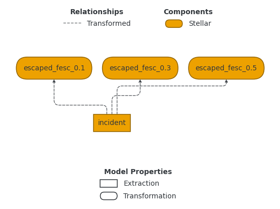
There are three escaped models now, one per escape fraction, each labelled with the value that made it. Notice there is still only one incident: the escape fraction is applied to the incident emission, so the extraction itself is unaffected and there is no reason to do it three times.

This is much easier to see than to describe, so let’s look at the model network. A family of variants is drawn as a single node badged with how many models it stands for, because an expansion of any size soon has more models than can be read at once. This one is small, so we can ask for all of them with show_variants.

expanded.plot_emission_graph(show_variants=True)

(<Figure size 534.872x393.056 with 1 Axes>, <Axes: >)

One extraction at the bottom feeding three independent chains. Every model downstream of the varied parameter is duplicated, and everything upstream is shared.

Sampling a distribution

Sometimes we don’t have a list of values in mind so much as a distribution to draw them from. ParameterDistribution covers that, and comes in a few flavours: ParameterUniformDist, ParameterNormalDist, ParameterLogUniformDist and ParameterLogNormalDist.

These take the number of values to draw and, optionally, a seed so the same models come back every time.

sampled = StellarEmissionModel(
    label="escaped",
    apply_to=incident,
    transformer=EscapingFraction(("fesc",)),
    fesc=ParameterNormalDist(
        0.3,
        0.08,
        n=4,
        seed=42,
        label_modifier="fesc_%.3f",
    ),
).expand_models()

for model in sampled.select("escaped*"):
    print(f"{model.label:18s} fesc = {model.variant_params['fesc']:.4f}")

escaped_fesc_0.217 fesc = 0.2168
escaped_fesc_0.324 fesc = 0.3244
escaped_fesc_0.360 fesc = 0.3600
escaped_fesc_0.375 fesc = 0.3752

The distribution is sampled once, up front, and then behaves exactly like a list of those values.

It is worth being clear about what is being sampled here. Each draw produces one model with one value, so four draws give four models. This is not a way of giving every particle its own escape fraction; if that is what you need, a ParameterFunction (see the custom models docs) computes a value per particle from the particle’s own properties.

Note also that the labels have to be unique, since they are the keys the emissions end up under. That means the label_modifier needs enough precision to tell the samples apart, which is why we used %.3f above rather than %.1f.

A distribution over a parameter which carries units needs to know what those units are, since the random number generators it samples with do not deal in quantities. State the bounds as quantities and it takes the units from them:

from unyt import kelvin

from synthesizer.emission_models.parameters import ParameterUniformDist

temperatures = ParameterUniformDist(
    20 * kelvin,
    60 * kelvin,
    n=3,
    seed=42,
    label_modifier="T%dK",
)

print(temperatures.realise().values)

[unyt_quantity(50.95824194, 'K'), unyt_quantity(37.55513759, 'K'), unyt_quantity(54.3439168, 'K')]

Or give the units separately and state the bounds as plain numbers, which is the only option for the log space flavours: their mean and sigma are in log10 space, so they cannot carry the units of a sample.

from synthesizer.emission_models.parameters import ParameterLogNormalDist

log_temperatures = ParameterLogNormalDist(
    1.5,
    0.1,
    n=3,
    seed=42,
    label_modifier="T%dK",
    units=kelvin,
)

print(log_temperatures.realise().values)

[unyt_quantity(33.92123909, 'K'), unyt_quantity(24.88866427, 'K'), unyt_quantity(37.58764527, 'K')]

Varying more than numbers

A variation does not have to be over a number, or even over a parameter value. The dust curve a model applies, or the generator it uses, can be varied in exactly the same way.

Here is the same model attenuated by three different dust curves where we use the aforementioned labels argument.

from synthesizer.emission_models import AttenuatedEmission
from synthesizer.emission_models.attenuation import Calzetti2000

attenuated = AttenuatedEmission(
    label="attenuated",
    apply_to=incident,
    emitter="stellar",
    tau_v=0.3,
    dust_curve=ParameterList(
        [PowerLaw(slope=-1), PowerLaw(slope=-0.7), Calzetti2000()],
        labels=["powerlaw_steep", "powerlaw_shallow", "calzetti"],
    ),
).expand_models()

for model in attenuated.select("attenuated*"):
    print(f"{model.label:28s} {type(model.transformer).__name__}")

attenuated_calzetti          Calzetti2000
attenuated_powerlaw_shallow  PowerLaw
attenuated_powerlaw_steep    PowerLaw

Generators work the same way, so a set of dust emission models is a variation like any other:

from synthesizer.emission_models import DustEmission
from synthesizer.emission_models.generators.dust.blackbody import Blackbody

# A plain attenuated model to balance the dust emission against
plain_attenuated = AttenuatedEmission(
    label="attenuated",
    apply_to=incident,
    emitter="stellar",
    tau_v=0.3,
    dust_curve=PowerLaw(slope=-1),
)

dust = DustEmission(
    dust_emission_model=ParameterList(
        [
            Blackbody(temperature=30 * kelvin),
            Greybody(temperature=30 * kelvin, emissivity=2.0),
            Greybody(temperature=60 * kelvin, emissivity=1.5),
        ],
        labels=["blackbody_30K", "greybody_30K", "greybody_60K"],
    ),
    emitter="stellar",
    label="dust_emission",
    dust_lum_intrinsic=incident,
    dust_lum_attenuated=plain_attenuated,
).expand_models()

for model in dust.select("dust_emission*"):
    print(f"{model.label:28s} {type(model.generator).__name__}")

dust_emission_blackbody_30K  Blackbody
dust_emission_greybody_30K   Greybody
dust_emission_greybody_60K   Greybody

Varying what a transformer or generator is made of

Swapping whole objects is the right thing when the alternatives are genuinely different curves. Often though we want the same curve with a different number in it: the slope of a power law, the temperature of a greybody, the position of the UV bump.

attenuated = AttenuatedEmission(
    label="attenuated",
    apply_to=incident,
    emitter="stellar",
    tau_v=0.3,
    dust_curve=PowerLaw(
        slope=ParameterList([-1.4, -1.0, -0.6], label_modifier="slope%.1f"),
    ),
).expand_models()

for model in attenuated.select("attenuated*"):
    print(f"{model.label:24s} {model.transformer}")

attenuated_slope-0.6     PowerLaw(slope=-0.6)
attenuated_slope-1.0     PowerLaw(slope=-1.0)
attenuated_slope-1.4     PowerLaw(slope=-1.4)

Anything the object holds can be varied this way, and generator arguments are no different from transformer ones.

Arguments which must carry units still must: the values inside a declaration are checked and converted just as a single value would be, so a list given in microns arrives in angstroms, and a list with a bare number in it is rejected where it was written rather than much later.

dust = DustEmission(
    dust_emission_model=Greybody(
        temperature=ParameterList(
            [20 * kelvin, 40 * kelvin, 60 * kelvin],
            label_modifier="T%dK",
        ),
        emissivity=2.0,
    ),
    emitter="stellar",
    label="dust_emission",
    dust_lum_intrinsic=incident,
    dust_lum_attenuated=plain_attenuated,
).expand_models()

for model in dust.select("dust_emission*"):
    print(f"{model.label:24s} {model.generator.temperature}")

dust_emission_T20K       20 K
dust_emission_T40K       40 K
dust_emission_T60K       60 K

Note that you can also vary a transformer or generator with different transformer or generator objects, and then vary the parameters of those objects as well. The expansion will find the parameters wherever they are, and duplicate the objects as needed.

Varying a premade model

Small models are useful for seeing what the machinery does, but the point of it is the big models.

PacmanEmission is a good test: it extracts the incident, transmitted and nebular emission, escapes a fraction of it, reprocesses the rest, attenuates that with a dust curve, and adds dust emission on top. That is a lot of models, and only some of them care about any given parameter.

Let’s vary two physically meaningful things at once: the escape fraction fesc, which controls how much light leaves without being reprocessed, and the optical depth tau_v, which controls how much of the reprocessed light the dust absorbs.

varied_pacman = PacmanEmission(
    grid,
    tau_v=ParameterList([0.1, 0.5, 1.0], label_modifier="tauv_%.1f"),
    fesc=ParameterList([0.0, 0.3], label_modifier="fesc_%.1f"),
    dust_curve=PowerLaw(slope=-1),
    dust_emission=Greybody(temperature=30 * kelvin, emissivity=2.0),
)

expanded_pacman = varied_pacman.expand_models()

print(f"before expanding: {len(varied_pacman._models)} models")
print(f"after expanding:  {len(expanded_pacman._models)} models")
print(
    f"building it once per combination would need "
    f"{6 * len(varied_pacman._models)} models"
)

before expanding: 14 models
after expanding:  38 models
building it once per combination would need 84 models

Six combinations of the two parameters, and yet nothing like six times the models. We can see why by counting how many variants each original model ended up with.

counts = Counter(
    model.variant_base or label for label, model in expanded_pacman.items()
)

for base, count in sorted(counts.items(), key=lambda kv: (-kv[1], kv[0])):
    print(f"{base:24s} x{count}")

attenuated               x6
dust_emission            x6
emergent                 x6
total                    x6
escaped                  x2
intrinsic                x2
reprocessed              x2
transmitted              x2
_nebular_line_no_fesc    x1
full_transmitted         x1
incident                 x1
nebular                  x1
nebular_continuum        x1
nebular_line             x1

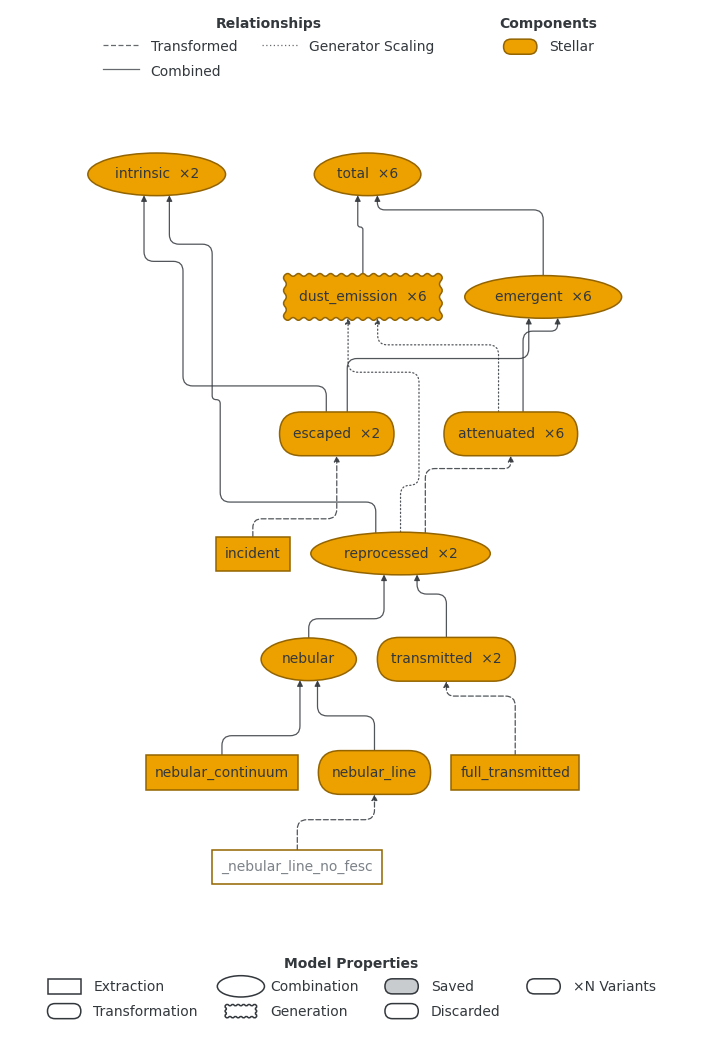
The grid extractions are there exactly once each. escaped, transmitted, reprocessed and intrinsic depend on the escape fraction but not on the optical depth, so there are two of each. attenuated depends on both, so it has all six, as do the dust_emission above it and the total at the top.

Note that we passed a single fesc to the model, and PacmanEmission handed it to several of its own models internally. Those are treated as one variation rather than one per model, so they vary in step and we get six combinations rather than a combination for every model that happened to receive it.

The network shows the shape of this rather better than a table does, and this is where the collapsed default earns its keep: each family is one node with its count, so the structure is legible however many variants there are.

expanded_pacman.plot_emission_graph()

(<Figure size 689.509x1017.12 with 1 Axes>, <Axes: >)

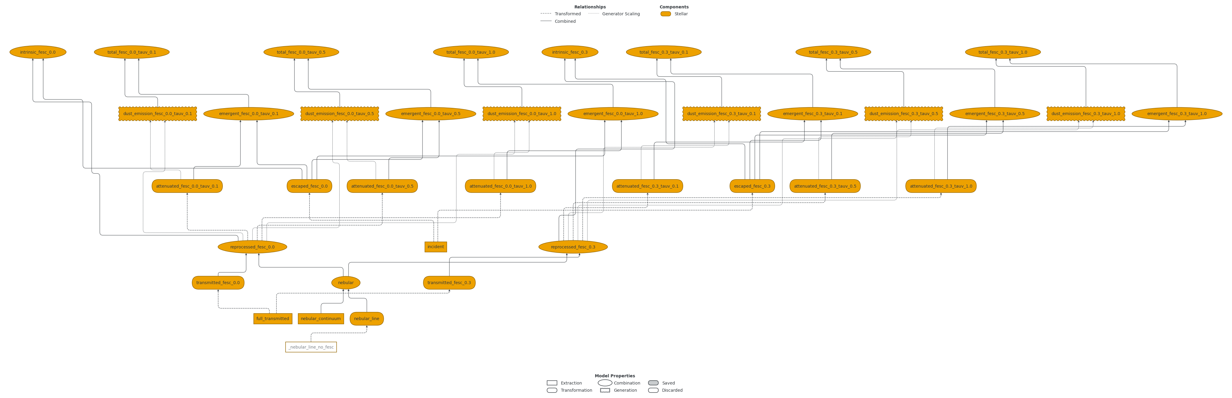
And the whole thing, with every variant drawn. Useful for a model this size, and rapidly useless beyond it.

expanded_pacman.plot_emission_graph(show_variants=True)

(<Figure size 4083.48x1308.79 with 1 Axes>, <Axes: >)

Generating the spectra

The expanded model is an ordinary emission model, so we use it exactly as we would any other. The important part is that this is a single get_spectra call: the shared models are computed once, and every variant is generated from them.

# A simple parametric galaxy to generate spectra for
stars = Stars(
    grid.log10ages,
    grid.metallicities,
    sf_hist=SFH.Constant(max_age=100 * Myr),
    metal_dist=ZDist.DeltaConstant(log10metallicity=-2.0),
    initial_mass=1e9 * Msun,
)
galaxy = Galaxy(stars)

galaxy.stars.get_spectra(expanded_pacman)

print(f"{len(galaxy.stars.spectra)} spectra on the component")

37 spectra on the component

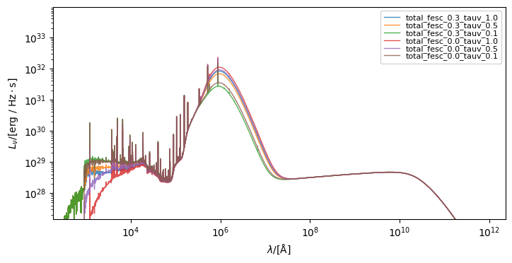
Each variant is stored under its own label, so we can pull out whichever ones we want to compare. Here is the total emission at each combination of the two parameters.

total = {
    model.label: galaxy.stars.spectra[model.label]
    for model in expanded_pacman.select("total*")
}

plot_spectra(total, figsize=(8, 5), quantity_to_plot="lnu")
plt.show()

Keeping the memory down

There is one thing to watch with a large expansion. A variant inherits every setting from the model it was copied from, saving included, so expansion does not change what is saved: it multiplies it. An EmissionModel saves its emission unless told otherwise, so unless we have already said which models we want, a large number of variants of a large model means a large number of spectra held on the component at once.

Saying so before expanding is inherited by every variant, which is usually what we want. Afterwards works too, and save_spectra accepts glob patterns, which is handy when the labels are generated rather than hand written.

expanded_pacman.save_spectra("total*")

print("saved:", sorted(expanded_pacman.saved_labels))

saved: ['total_fesc_0.0_tauv_0.1', 'total_fesc_0.0_tauv_0.5', 'total_fesc_0.0_tauv_1.0', 'total_fesc_0.3_tauv_0.1', 'total_fesc_0.3_tauv_0.5', 'total_fesc_0.3_tauv_1.0']

The intermediate models are still generated, since the total emission needs them, but their spectra are discarded as soon as nothing needs them any more rather than being kept to the end.

select is worth knowing about more generally: it matches models by glob and hands them back, so anything you would do to one model you can do to a family of them.

# Every model attenuated at a given optical depth, in one call
for model in expanded_pacman.select("attenuated*"):
    print(f"{model.label:24s} {model.variant_params}")

attenuated_fesc_0.0_tauv_0.1 {'fesc': 0.0, 'tau_v': 0.1}
attenuated_fesc_0.0_tauv_0.5 {'fesc': 0.0, 'tau_v': 0.5}
attenuated_fesc_0.0_tauv_1.0 {'fesc': 0.0, 'tau_v': 1.0}
attenuated_fesc_0.3_tauv_0.1 {'fesc': 0.3, 'tau_v': 0.1}
attenuated_fesc_0.3_tauv_0.5 {'fesc': 0.3, 'tau_v': 0.5}
attenuated_fesc_0.3_tauv_1.0 {'fesc': 0.3, 'tau_v': 1.0}