Line Ratios

The line_ratios submodule provides some helpful definitions that can be used to simplify calculating line ratios. As shown below, the submodule defines a set of commonly used ratios from the literature.

from synthesizer.emissions import line_ratios

print(line_ratios.available_ratios)

for ratio in line_ratios.available_ratios:
    print(
        f"{ratio} = {line_ratios.ratios[ratio][0]} "
        f"/ {line_ratios.ratios[ratio][1]}"
    )

('BalmerDecrement', 'N2', 'S2', 'O1', 'R2', 'R3', 'R23', 'O32', 'Ne3O2')
BalmerDecrement = H 1 6562.80A / H 1 4861.32A
N2 = N 2 6583.45A / H 1 6562.80A
S2 = S 2 6730.82A, S 2 6716.44A / H 1 6562.80A
O1 = O 1 6300.30A / H 1 6562.80A
R2 = O 2 3726.03A / H 1 4861.32A
R3 = O 3 5006.84A / H 1 4861.32A
R23 = O 3 4958.91A, O 3 5006.84A, O 2 3726.03A, O 2 3728.81A / H 1 4861.32A
O32 = O 3 5006.84A / O 2 3726.03A
Ne3O2 = Ne 3 3868.76A / O 2 3726.03A

Diagnostic Diagrams

In addition to line ratios, the submodule also provides a set of common diagnostic diagrams that can be used, for example, to classify the ionizing source.

print(line_ratios.available_diagrams)

for diagram in line_ratios.available_diagrams:
    print(
        f"{diagram} = {line_ratios.diagrams[diagram][0]} "
        f"/ {line_ratios.diagrams[diagram][1]}"
    )

('OHNO', 'BPT-NII', 'VO78-SII', 'VO78-OI')
OHNO = ['O 3 5006.84A', 'H 1 4861.32A'] / ['Ne 3 3868.76A', 'O 2 3726.03A, O 2 3728.81A']
BPT-NII = ['N 2 6583.45A', 'H 1 6562.80A'] / ['O 3 5006.84A', 'H 1 4861.32A']
VO78-SII = ['S 2 6730.82A, S 2 6716.44A', 'H 1 6562.80A'] / ['O 3 5006.84A', 'H 1 4861.32A']
VO78-OI = ['O 1 6300.30A', 'H 1 6562.80A'] / ['O 3 5006.84A', 'H 1 4861.32A']

Combining line_ratios with a LineCollection

from synthesizer.grid import Grid

grid = Grid("test_grid", "../../../tests/test_grid")
lines = grid.get_lines((1, 8))

As shown in the line collection docs, we can measure some predefined line ratios by passing the name of a ratio. We can also import all line ratios and loop over all pre-defined ratios.

for ratio_id in lines.available_ratios:
    ratio = lines.get_ratio(ratio_id)
    print(f"{ratio_id}: {ratio:.2f}")

BalmerDecrement: 2.93
N2: 0.07
S2: 0.07
O1: 0.00
R2: 0.76
R3: 3.82
R23: 6.48
O32: 5.00
Ne3O2: 0.23

Similarly, we can also do same for all the diagnostic diagrams.

for diagram_id in lines.available_diagrams:
    diagram0, diagram1 = lines.get_diagram(diagram_id)
    print(f"{diagram_id}: {diagram0:.2f} / {diagram1:.2f}")

OHNO: 3.82 / 0.13
BPT-NII: 0.07 / 3.82
VO78-SII: 0.07 / 3.82
VO78-OI: 0.00 / 3.82

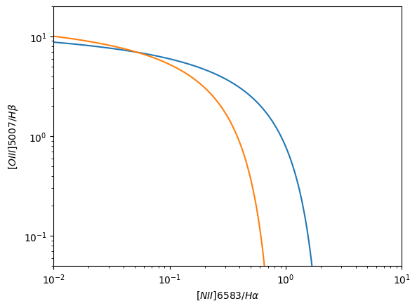
BPT Classification Regions

The lines_ratios module also provides functions defining BPT classification regions from Kewley+13 and Kauffmann+03. These functions take a set of x values and return the y values that define the classification regions.

import numpy as np

logNII_Ha = np.arange(-2.0, 1.0, 0.01)
logOIII_Hb_kewley = line_ratios.get_bpt_kewley01(logNII_Ha)
logOIII_Hb_kauffman = line_ratios.get_bpt_kauffman03(logNII_Ha)

We also provide functions to plot these classifications either on an existing set of axes or on a new figure.

fig, ax = line_ratios.plot_bpt_kewley01(
    logNII_Ha, show=False, fig=None, ax=None, label="Kewley+01"
)
_, _ = line_ratios.plot_bpt_kauffman03(
    logNII_Ha, fig=fig, ax=ax, label="Kauffman+03", show=True
)

/home/runner/work/synthesizer/synthesizer/src/synthesizer/emissions/line_ratios.py:178: RuntimeWarning: overflow encountered in power
  ax.loglog(10**logNII_Ha, 10**logOIII_Hb, **kwargs)
/home/runner/work/synthesizer/synthesizer/src/synthesizer/emissions/line_ratios.py:268: RuntimeWarning: overflow encountered in power
  ax.loglog(10**logNII_Ha, 10**logOIII_Hb, **kwargs)

For a more interesting example, see the metallicity dependence plots in the grid lines example.