Grid example
In this example we load a HDF5 (test) grid file into a corresponding Grid object, and use the inbuilt functionality to explore the grid.
[1]:
import matplotlib.pyplot as plt
import numpy as np
from matplotlib import colormaps as cm
from matplotlib.colors import Normalize
from unyt import angstrom

from synthesizer.grid import Grid
This object takes the location of the grids on your system (grid_dir) and the name of the grid you wish to load grid_name). Here we load a simple test grid provided with the module (hence the relative path).
[2]:
grid_dir = "../../../tests/test_grid"
grid_name = "test_grid"

grid = Grid(grid_name, grid_dir=grid_dir)
print(grid)
+--------------------------------------------------------------------------------+
|                                      GRID                                      |
+-----------------------------+--------------------------------------------------+
| Attribute                   | Value                                            |
+-----------------------------+--------------------------------------------------+
| grid_dir                    | '../../../tests/test_grid'                       |
+-----------------------------+--------------------------------------------------+
| grid_name                   | 'test_grid'                                      |
+-----------------------------+--------------------------------------------------+
| grid_ext                    | 'hdf5'                                           |
+-----------------------------+--------------------------------------------------+
| grid_filename               | '../../../tests/test_grid/test_grid.hdf5'        |
+-----------------------------+--------------------------------------------------+
| reprocessed                 | True                                             |
+-----------------------------+--------------------------------------------------+
| lines_available             | True                                             |
+-----------------------------+--------------------------------------------------+
| naxes                       | 2                                                |
+-----------------------------+--------------------------------------------------+
| date_created                | '2025-03-05'                                     |
+-----------------------------+--------------------------------------------------+
| synthesizer_grids_version   | '0.1.dev613+ga9a6aa9'                            |
+-----------------------------+--------------------------------------------------+
| synthesizer_version         | '0.8.5b1.dev124+ge16216b5'                       |
+-----------------------------+--------------------------------------------------+
| has_lines                   | True                                             |
+-----------------------------+--------------------------------------------------+
| has_spectra                 | True                                             |
+-----------------------------+--------------------------------------------------+
| lines_available             | True                                             |
+-----------------------------+--------------------------------------------------+
| ndim                        | 3                                                |
+-----------------------------+--------------------------------------------------+
| new_line_format             | True                                             |
+-----------------------------+--------------------------------------------------+
| nlam                        | 9244                                             |
+-----------------------------+--------------------------------------------------+
| nlines                      | 215                                              |
+-----------------------------+--------------------------------------------------+
| reprocessed                 | True                                             |
+-----------------------------+--------------------------------------------------+
| shape                       | (51, 13, 9244)                                   |
+-----------------------------+--------------------------------------------------+
| available_spectra           | [incident, linecont, nebular, transmitted,       |
|                             |  total, nebular_continuum]                       |
+-----------------------------+--------------------------------------------------+
| axes                        | [ages, metallicities]                            |
+-----------------------------+--------------------------------------------------+
| available_lines (215,)      | [He 2 1025.27A, O 6 1031.91A, O 6 1037.61A, ...] |
+-----------------------------+--------------------------------------------------+
| line_lams (215,)            | 1.03e+03 Å -> 2.48e+04 Å (Mean: 5.98e+03 Å)      |
+-----------------------------+--------------------------------------------------+
| incident_axes               | ['ages' 'metallicities']                         |
+-----------------------------+--------------------------------------------------+
| spec_names (4,)             | [incident, transmitted, nebular, ...]            |
+-----------------------------+--------------------------------------------------+
| lam (9244,)                 | 1.30e-04 Å -> 2.99e+11 Å (Mean: 9.73e+09 Å)      |
+-----------------------------+--------------------------------------------------+
| line_ids (215,)             | [He 2 1025.27A, O 6 1031.91A, O 6 1037.61A, ...] |
+-----------------------------+--------------------------------------------------+
| spectra                     | incident: ndarray                                |
|                             | linecont: ndarray                                |
|                             | nebular: ndarray                                 |
|                             | transmitted: ndarray                             |
|                             | total: ndarray                                   |
|                             | nebular_continuum: ndarray                       |
+-----------------------------+--------------------------------------------------+
| line_lums                   | nebular: unyt_array                              |
|                             | linecont: unyt_array                             |
|                             | nebular_continuum: unyt_array                    |
|                             | transmitted: unyt_array                          |
|                             | incident: unyt_array                             |
|                             | total: unyt_array                                |
+-----------------------------+--------------------------------------------------+
| line_conts                  | nebular: unyt_array                              |
|                             | linecont: unyt_array                             |
|                             | nebular_continuum: unyt_array                    |
|                             | transmitted: unyt_array                          |
|                             | incident: unyt_array                             |
|                             | total: unyt_array                                |
+-----------------------------+--------------------------------------------------+
| log10_specific_ionising_lum | HI: ndarray                                      |
|                             | HeII: ndarray                                    |
+-----------------------------+--------------------------------------------------+
A Grid can also take various arguments to limit the size of the grid, e.g. by isolating the Grid to a wavelength region of interest. This is particularly useful when making a large number of spectra from a high resolution Grid, where the memory footprint can become large.
Passing a wavelength array
If you only care about a grid of specific wavelength values, you can pass this array and the Grid will automatically be interpolated onto the new wavelength array using spectres:
[3]:
# Define a new set of wavelengths
new_lams = np.logspace(2, 5, 1000) * angstrom

# Create a new grid
grid = Grid(grid_name, grid_dir=grid_dir, new_lam=new_lams)
print(grid.shape)
(51, 13, 1000)
Passing wavelength limits
If you don’t want to modify the underlying grid resolution, but only care about a specific wavelength range, you can pass limits to truncate the grid at:
[4]:
# Create a new grid
grid = Grid(
    grid_name, grid_dir=grid_dir, lam_lims=(10**3 * angstrom, 10**4 * angstrom)
)
print(grid.shape)
(51, 13, 691)
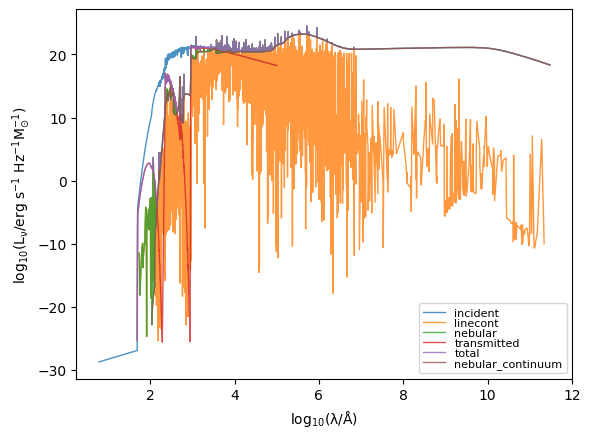
Plot a single grid point
We can plot the spectra at the location of a single point in our grid. First, we choose some age and metallicity
[5]:
# Return to the unmodified grid
grid = Grid(grid_name, grid_dir=grid_dir)

log10age = 6.0  # log10(age/yr)
Z = 0.01  # metallicity
We then get the index location of that grid point for this age and metallicity
[6]:
grid_point = grid.get_grid_point(log10ages=log10age, metallicity=Z)
We can then loop over the available spectra (contained in grid.spec_names) and plot
[7]:
for spectra_type in grid.available_spectra:
    # Get `Sed` object
    sed = grid.get_sed_at_grid_point(grid_point, spectra_type=spectra_type)

    # Mask zero valued elements
    mask = sed.lnu > 0
    plt.plot(
        np.log10(sed.lam[mask]),
        np.log10(sed.lnu[mask]),
        lw=1,
        alpha=0.8,
        label=spectra_type,
    )

plt.legend(fontsize=8, labelspacing=0.0)
plt.xlabel(r"$\rm log_{10}(\lambda/\AA)$")
plt.ylabel(r"$\rm log_{10}(L_{\nu}/erg\ s^{-1}\ Hz^{-1} M_{\odot}^{-1})$")
[7]:
Text(0, 0.5, '$\\rm log_{10}(L_{\\nu}/erg\\ s^{-1}\\ Hz^{-1} M_{\\odot}^{-1})$')
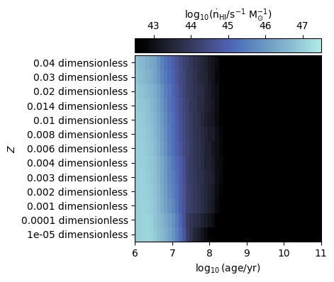
Plot ionising luminosities
We can also plot properties over the entire age and metallicity grid, such as the ionising luminosity.
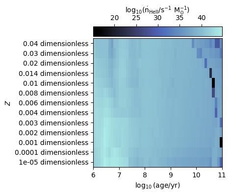
In the examples below we plot ionising luminosities for HI and HeII
[8]:
fig, ax = grid.plot_specific_ionising_lum(ion="HI")
[9]:
fig, ax = grid.plot_specific_ionising_lum(ion="HeII")
Resampling Grids
If you want to resample a grid after instantiation, you can apply the intrep_spectra method:
[10]:
# Define a new set of wavelengths
new_lams = np.logspace(2, 5, 10000) * angstrom

print("The old grid had dimensions:", grid.spectra["incident"].shape)

# Get the grid interpolated onto the new wavelength array
grid.interp_spectra(new_lam=new_lams)

print("The interpolated grid has dimensions:", grid.spectra["incident"].shape)
The old grid had dimensions: (51, 13, 9244)
The interpolated grid has dimensions: (51, 13, 10000)
Note that this will overwrite the spectra and wavelengths read from the file in place. To get back to the original arrays, a separate Grid can be instatiated without the modified wavelength array.
Collapsing Grids
While most of the models within synthesizer are capable of handling higher dimensionality grids (i.e. grids with more dimensions than age and metallicity), other workflows might require some method to reduce the dimensionality.
This functionality is provided via the collapse() method, which collapses the grid over a specified axis. There are three ways to actually collapse the grid, specified by the method keyword argument:
marginalizeover the entire axis. This is useful if you don’t know anything about this parameter, and just want to adopt the average over it. You can specify the function used to marginalize with the keyword argumentmarginalize_function; the default isnp.average.Pick the value
nearestto a specified value. If you know the value of the parameter you want to use, you can collapse the grid by picking the value closest to your specified value. For this, you need to specify thevaluekeyword argument.interpolateto a specified value. Similar tonearest, but with a linear interpolation to your specifiedvalue. This is useful in workflows where you can’t adopt a discrete value, but be warned that interpolating over a coarse grid can give unrealistic results. You can apply a transformation to the axis before interpolating, e.g. to interpolate in log-space rather than linear space, with the keyword argumentpre_interp_function.
For example, here we collapse the grid over the metallicity axis:
[11]:
print("The old grid had dimensions:", grid.spectra["incident"].shape)
print("and axes:", ", ".join(grid.axes))

# Collapse the grid to a single metallicity value
grid.collapse("metallicities", value=0.03, method="nearest")

print("The collapsed grid has dimensions:", grid.spectra["incident"].shape)
print("and axes:", ", ".join(grid.axes))
The old grid had dimensions: (51, 13, 10000)
and axes: ages, metallicities
The collapsed grid has dimensions: (51, 10000)
and axes: ages
Note that collapse() will overwrite the Grid in place. You can restore the grid to its original dimensionality by re-loading from the HDF5 file:
[12]:
# Re-load the original grid
grid = Grid(grid_name, grid_dir=grid_dir)
Converting a Grid into an Sed
Any of the spectra arrays stored within a Grid can be returned as Sed objects (see the Sed docs). This enables all of the analysis methods provide on an Sed to be used on the whole spectra grid. To do this we simply call get_sed with the spectra type we want to extract, and then use any of the included methods.
[13]:
# Get the sed object
sed = grid.get_sed(spectra_type="incident")

# Measure the balmer break for all spectra in the grid (limiting the output)
sed.measure_balmer_break()[5:10, 5:10]
[13]:
array([[0.98984907, 1.0073854 , 1.00280181, 0.99874568, 0.94231088],
       [1.01585662, 1.01514631, 1.00152695, 0.97659766, 0.97649268],
       [1.04604272, 1.03708356, 1.02677301, 1.00043255, 0.98165109],
       [1.12498086, 1.07987898, 1.05375405, 1.01931841, 1.01376902],
       [1.09541215, 1.06731203, 1.05205108, 1.04534501, 1.03791808]])
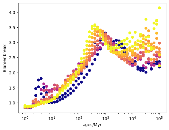
Working with flattened grids
Sometimes it’s useful to work with flattened (i.e. one dimensional) versions of a grid of spectra, photometry etc. To facilitate this the get_flattened_axes_values method on grid can be used to get the flattend axes values.
[14]:
cm["plasma"](0.5)
[14]:
(np.float64(0.798216),
 np.float64(0.280197),
 np.float64(0.469538),
 np.float64(1.0))
[15]:
grid._axes_units["ages"]
grid._axes_values["ages"]
[15]:
array([1.00000000e+06, 1.25892541e+06, 1.58489319e+06, 1.99526231e+06,
       2.51188643e+06, 3.16227766e+06, 3.98107171e+06, 5.01187234e+06,
       6.30957344e+06, 7.94328235e+06, 1.00000000e+07, 1.25892541e+07,
       1.58489319e+07, 1.99526231e+07, 2.51188643e+07, 3.16227766e+07,
       3.98107171e+07, 5.01187234e+07, 6.30957344e+07, 7.94328235e+07,
       1.00000000e+08, 1.25892541e+08, 1.58489319e+08, 1.99526231e+08,
       2.51188643e+08, 3.16227766e+08, 3.98107171e+08, 5.01187234e+08,
       6.30957344e+08, 7.94328235e+08, 1.00000000e+09, 1.25892541e+09,
       1.58489319e+09, 1.99526231e+09, 2.51188643e+09, 3.16227766e+09,
       3.98107171e+09, 5.01187234e+09, 6.30957344e+09, 7.94328235e+09,
       1.00000000e+10, 1.25892541e+10, 1.58489319e+10, 1.99526231e+10,
       2.51188643e+10, 3.16227766e+10, 3.98107171e+10, 5.01187234e+10,
       6.30957344e+10, 7.94328235e+10, 1.00000000e+11])
[16]:
# Get the balmer breaks of the entire grid
balmer_breaks = sed.measure_balmer_break()

# Get a flattened version of the Balmer break grid
flattened_balmer_breaks = balmer_breaks.flatten()

# Get the flattened version of the axes
flattend_axes_values = grid.get_flattened_axes_values()

# Normlise metallicities and create an array of colors
norm = Normalize(vmin=-4, vmax=-1.5, clip=True)
colors = cm["plasma"](norm(np.log10(flattend_axes_values["metallicities"])))

# Plot
plt.scatter(
    flattend_axes_values["ages"].to("Myr").value,
    flattened_balmer_breaks,
    c=colors,
)
plt.xscale("log")
plt.xlabel("ages/Myr")
plt.ylabel("Blamer break")
plt.show()