Online Training
A variation of SBI is Sequential Neural Posterior Estimation (SNPE), where the model is trained online, i.e., in multiple rounds. In each round, simulations are generated from the current posterior estimate, and the model is updated with these new simulations. This approach can be more efficient in terms of simulation budget, especially when the prior is broad and the posterior is narrow.
However, the model is no longer amortized, as it is specialized to the specific observation after training. This means that a new model must be trained for each new observation, which can be computationally expensive if many observations need to be analyzed.
[1]:
from synference import SBI_Fitter, test_data_dir

fitter = SBI_Fitter.init_from_hdf5(
    model_name="test", hdf5_path=f"{test_data_dir}/example_model_library.hdf5"
)

fitter.create_feature_array();
/opt/hostedtoolcache/Python/3.10.20/x64/lib/python3.10/site-packages/tqdm/auto.py:21: TqdmWarning: IProgress not found. Please update jupyter and ipywidgets. See https://ipywidgets.readthedocs.io/en/stable/user_install.html
  from .autonotebook import tqdm as notebook_tqdm
2026-06-24 09:47:11,572 | synference | INFO     | ---------------------------------------------
2026-06-24 09:47:11,573 | synference | INFO     | Features: 8 features over 100 samples
2026-06-24 09:47:11,573 | synference | INFO     | ---------------------------------------------
2026-06-24 09:47:11,574 | synference | INFO     | Feature: Min - Max
2026-06-24 09:47:11,575 | synference | INFO     | ---------------------------------------------
2026-06-24 09:47:11,575 | synference | INFO     | JWST/NIRCam.F070W: 7.131974 - 42.758 AB
2026-06-24 09:47:11,576 | synference | INFO     | JWST/NIRCam.F090W: 7.108530 - 39.933 AB
2026-06-24 09:47:11,577 | synference | INFO     | JWST/NIRCam.F115W: 7.012560 - 38.354 AB
2026-06-24 09:47:11,577 | synference | INFO     | JWST/NIRCam.F150W: 6.969396 - 36.997 AB
2026-06-24 09:47:11,578 | synference | INFO     | JWST/NIRCam.F200W: 7.133157 - 35.470 AB
2026-06-24 09:47:11,578 | synference | INFO     | JWST/NIRCam.F277W: 7.670149 - 33.243 AB
2026-06-24 09:47:11,579 | synference | INFO     | JWST/NIRCam.F356W: 8.072730 - 32.490 AB
2026-06-24 09:47:11,580 | synference | INFO     | JWST/NIRCam.F444W: 8.353975 - 31.965 AB
2026-06-24 09:47:11,580 | synference | INFO     | ---------------------------------------------
Now we will recreate the simulator from the library data stored in the HDF5 file.
[2]:
fitter.recreate_simulator_from_library(
    override_library_path=f"{test_data_dir}/example_model_library.hdf5",
    override_grid_path="test_grid.hdf5",
);
2026-06-24 09:47:11,592 | synference | INFO     | Overriding internal library name from provided file path.
2026-06-24 09:47:11,822 | synference | INFO     | Simulator recreated from library at /home/runner/.local/share/Synthesizer/data/synference/example_model_library.hdf5.
Now we can choose an observation for our multiple rounds of online training. Here, we will randomly select one of the simulations from our library as the observation.
[3]:
index = 20
sample = fitter.feature_array[index]
true_params = fitter.fitted_parameter_array[index]

sample
[3]:
array([28.922905, 27.99003 , 27.05276 , 26.493101, 25.965355, 25.390919,
       24.99644 , 24.839458], dtype=float32)
Now we can run our online SBI model - to do this we set learning_type to ‘online’, specify the number of online rounds with ‘num_online_rounds’, and provide our chosen observation with ‘online_training_xobs’. We also set the number of simulations per round with ‘num_simulations’. The engine is set to ‘SNPE’ to use Sequential Neural Posterior Estimation, but SNLE and SNRE are also available for online training.
[4]:
fitter.run_single_sbi(
    online_training_xobs=sample,
    learning_type="online",
    engine="SNPE",
    num_simulations=1000,
    num_online_rounds=4,
    override_prior_ranges={"peak_age": (10, 1000)},
    evaluate_model=False,
    plot=False,
);
2026-06-24 09:47:11,841 | synference | INFO     | ---------------------------------------------
2026-06-24 09:47:11,842 | synference | INFO     | Prior ranges:
2026-06-24 09:47:11,842 | synference | INFO     | ---------------------------------------------
2026-06-24 09:47:11,844 | synference | INFO     | redshift: 0.00 - 4.98 [dimensionless]
2026-06-24 09:47:11,845 | synference | INFO     | log_mass: 8.01 - 11.99 [log10_Msun]
2026-06-24 09:47:11,846 | synference | INFO     | tau_v: 0.01 - 3.00 [mag]
2026-06-24 09:47:11,847 | synference | INFO     | tau: 0.11 - 1.98 [dimensionless]
2026-06-24 09:47:11,849 | synference | INFO     | peak_age: 10.00 - 1000.00 [Myr]
2026-06-24 09:47:11,849 | synference | INFO     | log10metallicity: -3.98 - -1.41 [log10(Zmet)]
2026-06-24 09:47:11,850 | synference | INFO     | ---------------------------------------------
2026-06-24 09:47:11,851 | synference | INFO     | Processing prior...
2026-06-24 09:47:11,854 | synference | INFO     | Using provided xobs for online training: (8,)
Wrapping GalaxySimulator for SBI...
2026-06-24 09:47:11,856 | synference | INFO     | Creating mdn network with SNPE engine and sbi backend.
2026-06-24 09:47:11,856 | synference | INFO     |      hidden_features: 50
2026-06-24 09:47:11,857 | synference | INFO     |      num_components: 4
2026-06-24 09:47:11,858 | synference | INFO     | Training on cpu.
INFO:root:MODEL INFERENCE CLASS: SNPE
INFO:root:The first round of inference will simulate from the given proposal or prior.
Running 1000 simulations.: 100%|██████████| 1000/1000 [00:39<00:00, 25.51it/s]
INFO:root:Running round 1 / 4
INFO:root:Training model 1 / 1.
Neural network successfully converged after 839 epochs.
1110it [00:00, 424284.83it/s]
Running 1000 simulations.: 100%|██████████| 1000/1000 [00:31<00:00, 32.00it/s]
INFO:root:Running round 2 / 4
INFO:root:Training model 1 / 1.
Using SNPE-C with atomic loss
 Neural network successfully converged after 55 epochs.
1374it [00:00, 333466.83it/s]
Running 1000 simulations.: 100%|██████████| 1000/1000 [00:35<00:00, 27.92it/s]
INFO:root:Running round 3 / 4
INFO:root:Training model 1 / 1.
Using SNPE-C with atomic loss
 Neural network successfully converged after 15 epochs.
1552it [00:00, 314107.31it/s]
Running 1000 simulations.: 100%|██████████| 1000/1000 [00:34<00:00, 29.35it/s]
INFO:root:Running round 4 / 4
INFO:root:Training model 1 / 1.
Using SNPE-C with atomic loss
 Training neural network. Epochs trained: 14
INFO:root:It took 168.16912269592285 seconds to train models.
INFO:root:Saving model to /opt/hostedtoolcache/Python/3.10.20/x64/lib/python3.10/models/test
 Neural network successfully converged after 15 epochs.2026-06-24 09:50:39,261 | synference | INFO     | Time to train model(s): 0:03:27.420449
2026-06-24 09:50:39,280 | synference | INFO     | Saved model parameters to /opt/hostedtoolcache/Python/3.10.20/x64/lib/python3.10/models/test/test_20260624_094711_params.pkl.
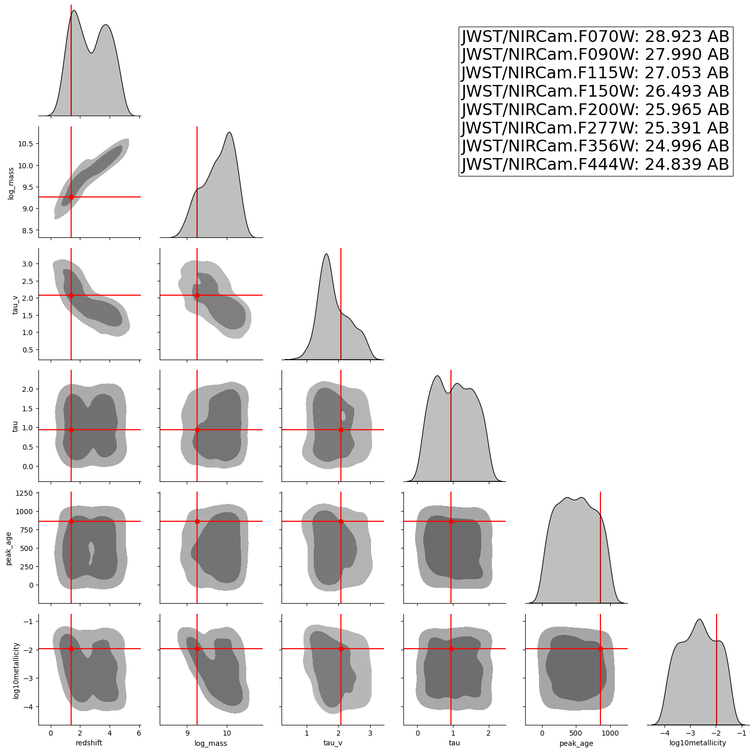
Now we can specifically see how the model performs on the conditioned observation.
[5]:
samples = fitter.sample_posterior(X_test=sample)

fitter.plot_posterior(
    X=sample,
    y=samples,
    num_samples=1000,
)
30s per sample.
Sampling from posterior: 100%|██████████| 1/1 [00:00<00:00, 206.57it/s]
2026-06-24 09:50:39,298 | synference | INFO     | [  1.40883327   9.2566061    2.07742095   0.93622267 862.08276367
  -1.96798372]
1509it [00:00, 305448.81it/s]
INFO:root:Saving single posterior plot to /opt/hostedtoolcache/Python/3.10.20/x64/lib/python3.10/models/test/plots/test_0_plot_single_posterior.jpg...
[5]:
<seaborn.axisgrid.PairGrid at 0x7fa3251404f0>