Noise Modelling

Here we will look at the noise modelling - how to generate a noise model, and how to use it in training.

All noise models have certain basic characteristics:

• They take in a set of fluxes (or other features) and return noisy fluxes. If return_noise=True, they also return the standard deviation of the noise applied to each flux or an estimate thereof given the scattered flux itself.

• They can be serialized to HDF5 files for later use, and restored from such files. This uses the serialize_to_hdf5 method and the load_unc_model_from_hdf5 factory function.

Depth Noise Model

The simplest noise model is the Depth Noise Model, which adds Gaussian noise with a standard deviation determined by the depth of the observation. This takes a depth (in AB mag), and optionally a depth sigma (default 5.0), which sets the SNR at the given depth. The flux is this noise model is distributed in flux space not magnitude space.

If you’re using this model there are a few things to keep in mind:

• If you are training in magnitude space and conditioning the model on the magnitude errors, they are not well-behaved near the detection limit, as the flux errors become non-Gaussian in magnitude space. The code uses the approximation sigma_mag = 2.5 / ln(10) * (sigma_flux / flux) to estimate the magnitude errors, but this breaks down near the detection limit, and can lead to very large or undefined magnitude errors. Negative fluxes will lead to NaN magnitude errors, as they can’t be representing logarithmically.

import matplotlib.pyplot as plt
import numpy as np
from unyt import nJy

from synference import DepthUncertaintyModel

noise_model = DepthUncertaintyModel(depth_ab=28, return_noise=True)


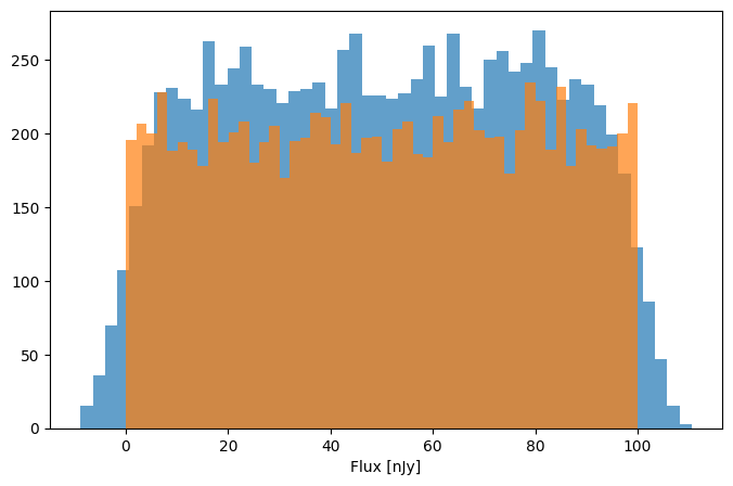
fluxes = np.random.uniform(0.1, 100, size=10_000) * nJy

noisy_fluxes, sigmas = noise_model.apply_noise(fluxes, out_units=nJy)

plt.figure(figsize=(8, 5))
plt.xlabel("Flux [nJy]")
plt.hist(
    (noisy_fluxes),
    bins=50,
    density=False,
    alpha=0.7,
)

plt.hist(
    (fluxes.to_value(nJy)),
    bins=50,
    density=False,
    alpha=0.7,
);

/opt/hostedtoolcache/Python/3.10.19/x64/lib/python3.10/site-packages/tqdm/auto.py:21: TqdmWarning: IProgress not found. Please update jupyter and ipywidgets. See https://ipywidgets.readthedocs.io/en/stable/user_install.html
  from .autonotebook import tqdm as notebook_tqdm

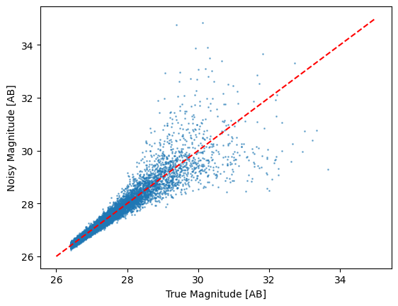
We can set the output units as well - here we choose AB magnitudes, and plot the noisy fluxes against the true fluxes:

noisy_fluxes, sigmas = noise_model.apply_noise(fluxes, out_units="AB")


plt.scatter(-2.5 * np.log10(fluxes) + 31.4, noisy_fluxes, s=1, alpha=0.5)
# plot 1:1 line
plt.plot([26, 35], [26, 35], color="red", linestyle="--")
plt.xlabel("True Magnitude [AB]")
plt.ylabel("Noisy Magnitude [AB]")

Text(0, 0.5, 'Noisy Magnitude [AB]')

General Noise Model

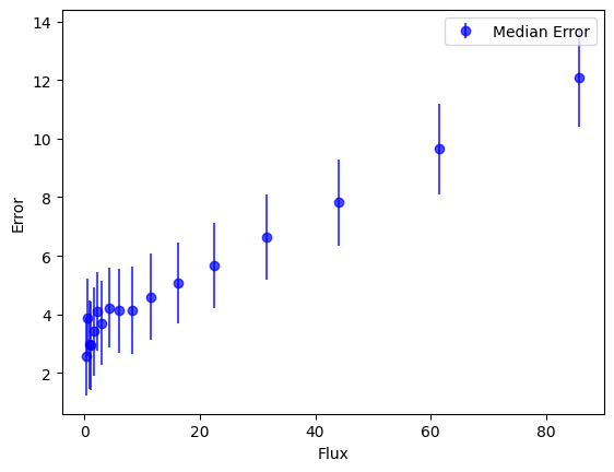
This noise model is designed to match the noise distribution of a given dataset. It fits a model to the relationship between flux and flux uncertainty in the data, and uses this to generate noisy fluxes. There are a few different ways to use this model, depending on your use case.

from synference import GeneralEmpiricalUncertaintyModel

# Generate some fake random data with noise

# model error as a function of flux in bins
errors = 0.1 * fluxes + 1.0 * nJy + 5.0 * nJy * np.random.rand(len(fluxes))


noise_model = GeneralEmpiricalUncertaintyModel(
    observed_fluxes=fluxes, observed_errors=errors, flux_unit=nJy
)

noise_model.plot()

Asinh Noise Model

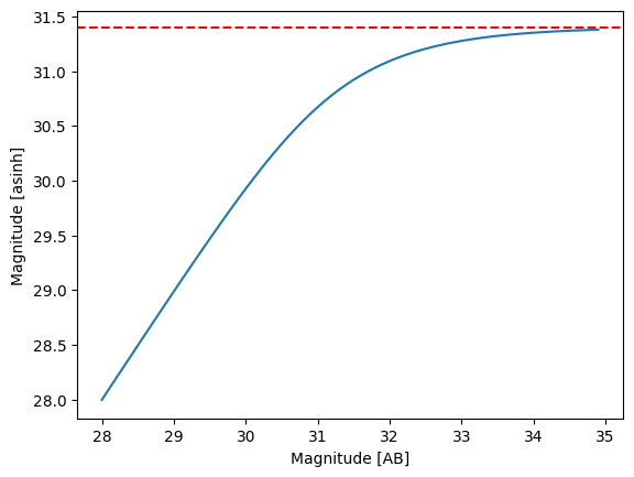
This noise model can also match the noise distribution of a given dataset, but uses an asinh transformation to better handle low SNR data. This is particularly useful when working with data that includes many non-detections or upper limits. The asinh transformation helps to stabilize the variance and make the noise distribution more Gaussian-like, which can improve the performance of models trained on this data.

from synference.utils import f_jy_err_to_asinh, f_jy_to_asinh

mags = np.arange(28, 35, 0.1)
fluxes = 10 ** ((mags - 31.4) / -2.5) * nJy
asinh_fluxes = f_jy_to_asinh(fluxes.to("Jy"), f_b=1 * nJy)

plt.plot(mags, asinh_fluxes)
plt.axhline(31.4, color="red", linestyle="--")
plt.xlabel("Magnitude [AB]")
plt.ylabel("Magnitude [asinh]")

Text(0, 0.5, 'Magnitude [asinh]')

This noise model is implemented in the AsinhEmpiricalUncertaintyModel class. It works similarly to the GeneralEmpiricalUncertaintyModel, but applies the asinh transformation to the fluxes before fitting the noise model. It only excepts input fluxes in Jy units, and whilst the apply_noise method will accept the out_flux_unit argument for consistency with other noise models, the output fluxes will always be in asinh magnitudes.

For this model, the asinh softening parameter is not set directly, but in multiples of the median standard deviation of the flux uncertainties in the training data. This is set using the f_b_factor argument when initializing the model. For example, setting f_b_factor=1.0 will set the softening parameter to the median flux uncertainty, while f_b_factor=2.0 will set it to twice the median flux uncertainty. By default, f_b_factor=5.0, so the softening parameter is set to five times the median flux uncertainty (aka the \(5\sigma\) detection limit).

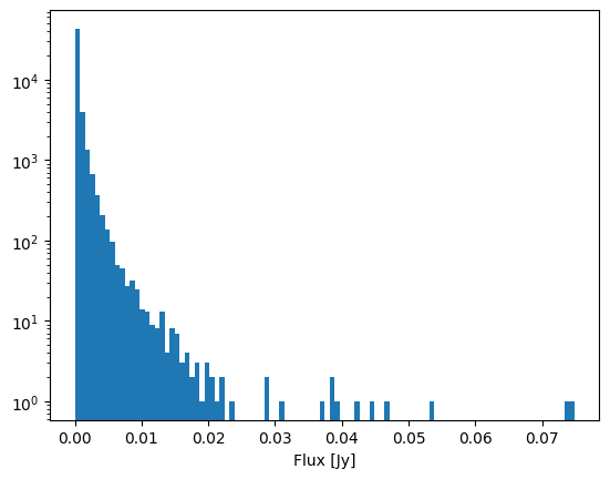
For this example we setup a more realstic scenario, with a catalogue of 50,000 fake sources with a fixed background level, a fractioanl error and an overall lognormal flux distribution.

from synference import AsinhEmpiricalUncertaintyModel
from synference.utils import f_jy_to_asinh

# --- 1. Define Realistic Survey Parameters ---
N_SOURCES: int = 50_000

# Background noise limit (e.g., 100 uJy).
# This dominates the error for faint sources.
BACKGROUND_NOISE_JY: float = 0.0001

# Fractional/calibration error (e.g., 2%).
# This dominates the error for bright sources.
FRACTIONAL_ERROR: float = 0.02

# Log-normal distribution parameters for "true" fluxes.
# We set the median flux to be near the noise floor.
FLUX_MEDIAN_JY: float = 0.00015
FLUX_LOG_SIGMA: float = 1.5  # Width of the log-normal distribution

# --- 2. Generate "True" Fluxes ---
# Use a log-normal distribution: many faint sources, few bright ones
true_flux_jy = np.random.lognormal(
    mean=np.log(FLUX_MEDIAN_JY), sigma=FLUX_LOG_SIGMA, size=N_SOURCES
)

# --- 3. Calculate "Ideal" Error for Each True Flux ---
# This is the characteristic error model: sqrt(bg_noise^2 + (frac_err * flux)^2)
ideal_error_jy = np.sqrt(BACKGROUND_NOISE_JY**2 + (FRACTIONAL_ERROR * true_flux_jy) ** 2)

# --- 4. Simulate "Observed" Fluxes by Scattering by the Error ---
# The observed flux is the true flux plus Gaussian noise
observed_flux_jy = true_flux_jy + np.random.normal(loc=0.0, scale=ideal_error_jy, size=N_SOURCES)

# The "observed error" is the error the pipeline *reports*.
# We assume the pipeline correctly estimates the ideal error.
observed_error_jy = ideal_error_jy

# Plot a flux histogram
plt.hist(true_flux_jy, label="Fluxes", bins=100)
plt.yscale("log")
plt.xlabel("Flux [Jy]")

Text(0.5, 0, 'Flux [Jy]')

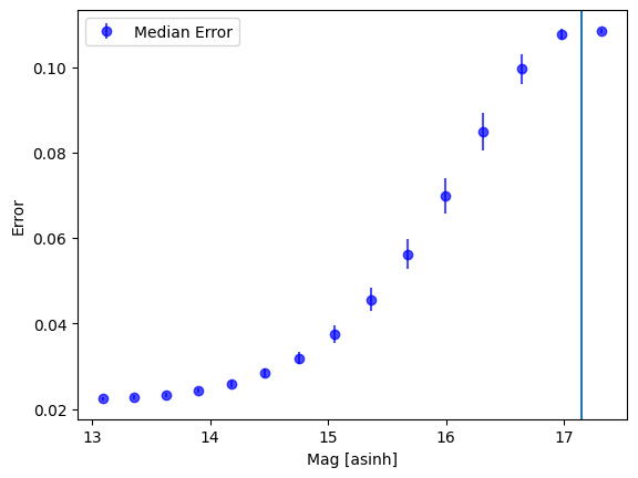
From this realistic dataset we can generate our AsinhEmpiricalUncertaintyModel. Note that some datapoints fall below the softening parameter - these are originally negative fluxes which can be represented by asinh magnitudes.

noise_model = AsinhEmpiricalUncertaintyModel(
    observed_phot_jy=observed_flux_jy,
    observed_phot_errors_jy=observed_error_jy,
)

print(noise_model.b)

# plot noise_model.b
fig, ax = plt.subplots()
noise_model.plot(ax=ax)


plt.axvline(f_jy_to_asinh(noise_model.b))

0.0005002284059637181 Jy

<matplotlib.lines.Line2D at 0x7fd7921b54e0>

?truncnorm

Object `truncnorm` not found.

Example Noise Models for Real Data

Let’s try making noise models for some real data. We will use the UNCOVER DR3 catalog (0.32” apertures) for this example. First, we need to download the catalog.

direct_link = r"https://drive.google.com/uc?export=download&id=1dDo2RhiP_OCjO5hEc90T8HnnC0lYxqfl"
file_name = r"UNCOVER_DR3_LW_D140_catalog.fits"
import os
import subprocess

if not os.path.exists(file_name):
    subprocess.run(
        ["wget", direct_link, "-O", file_name], stdout=subprocess.DEVNULL, stderr=subprocess.DEVNULL
    )

from astropy.table import Table

catalog = Table.read("UNCOVER_DR3_LW_D140_catalog.fits")

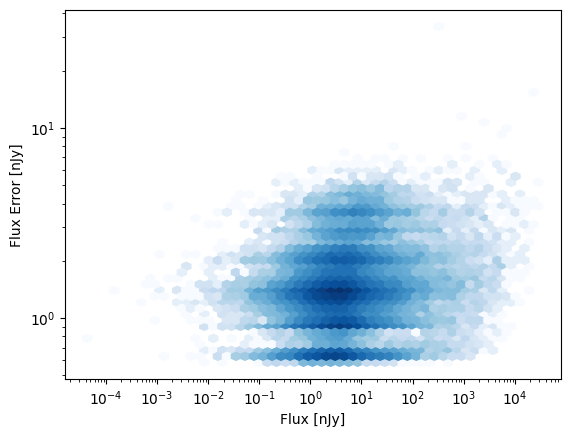
Here for the F444W band is the flux error as a function of flux, for the full catalog. (Note fluxes are in 10xnJy units in the catalog.)

import numpy as np
from matplotlib import pyplot as plt

flux = list(catalog["f_f444w"].value) * 10 * nJy
flux_err = list(catalog["e_f444w"].value) * 10 * nJy

mask = (flux > 0) & (flux_err > 0)
flux = flux[mask]
flux_err = flux_err[mask]

plt.hexbin(
    flux, flux_err, gridsize=50, cmap="Blues", mincnt=1, yscale="log", xscale="log", norm="log"
)
plt.xlabel("Flux [nJy]")
plt.ylabel("Flux Error [nJy]")

Text(0, 0.5, 'Flux Error [nJy]')

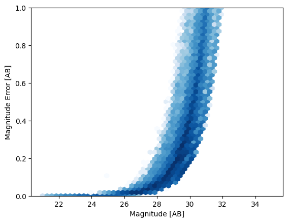
In magnitude space, this looks like the following. It’s worth noting that the magnitude errors become asymmetric and non-Gaussian near the detection limit, which can cause issues if you’re training in magnitude space and conditioning on the magnitude errors.

mag = -2.5 * np.log10(flux / 3631e9)
mag_err = (2.5 / np.log(10)) * (flux_err / flux)

plt.hexbin(mag, mag_err, gridsize=50, cmap="Blues", mincnt=1, norm="log", extent=(21, 35, 0, 1))
plt.xlabel("Magnitude [AB]")
plt.ylabel("Magnitude Error [AB]")
plt.ylim(0, 1)

(0.0, 1.0)

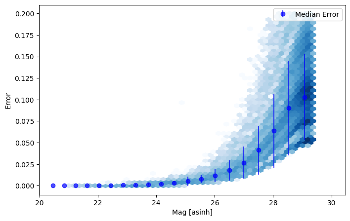
Now we can plot the asinh uncertainty model fit for the F444W band, on top of the data.

nm = AsinhEmpiricalUncertaintyModel(
    observed_phot_jy=flux,
    observed_phot_errors_jy=flux_err,
)
print(f"The derived softening parameter is b = {nm.b:.3e}")
fig, ax = plt.subplots(figsize=(8, 5))

true_f_asinh = f_jy_to_asinh(flux, f_b=nm.b)

true_f_err_asinh = f_jy_err_to_asinh(flux, flux_err, f_b=nm.b)

ax.hexbin(
    true_f_asinh,
    true_f_err_asinh,
    gridsize=50,
    cmap="Blues",
    mincnt=1,
    norm="log",
    extent=(21, 30, 0, 0.2),
)

nm.plot(ax=ax)

The derived softening parameter is b = 6.654e+00 nJy