Basic Library Generation
Now that we have a basic understanding of how to use Synthesizer to create a galaxy object, we can move on to generating a library of galaxies. This is done using the GalaxyBasis class within Synference, which takes a set of parameters and generates a library of galaxies based on those parameters.
In the simplest scenario, you define the parameter space you want to sample outside of the GalaxyBasis object. You then initialize the GalaxyBasis using these arrays.
We provide helper functions to generate these arrays for you, but you have complete flexibility to define your own, more complex parameter spaces if you wish.
Drawing Samples
[1]:
%load_ext autoreload
%autoreload 2

from matplotlib import pyplot as plt

from synference import GalaxyBasis
/opt/hostedtoolcache/Python/3.10.20/x64/lib/python3.10/site-packages/tqdm/auto.py:21: TqdmWarning: IProgress not found. Please update jupyter and ipywidgets. See https://ipywidgets.readthedocs.io/en/stable/user_install.html
  from .autonotebook import tqdm as notebook_tqdm
These arrays can be generated using the draw_from_hypercube function, which takes as input the number of samples you want to draw, and a dictionary of parameter ranges. In this dictionary, the key is the parameter range, and the value is a tuple defining the minimum and maximum value for that parameter. The function will then return a dictionary of arrays, where each array contains the sampled values for each parameter. Other sampling schemes can be used (e.g. a Sobol
sequence)
By default, the draw_from_hypercube function uses a form of low-discrepancy sampling called Latin Hypercube Sampling (LHS). LHS is highly efficient compared to random sampling, especially when dealing with many parameters, as it ensures that the parameter space is sampled more evenly.
The dictionary we must define encapsulates our prior knowledge about the parameter space we intend to sample.
For this example, we will define a parameter space with two parameters: redshift and log_stellar_mass. The default sampling method is uniform sampling between the upper and lower bounds provided, but you can draw from any distribution you like by defining the arrays yourself.
[2]:
from synference import draw_from_hypercube

param_ranges = {"redshift": (0.0, 5.0), "log_stellar_mass": (8.0, 12.0)}
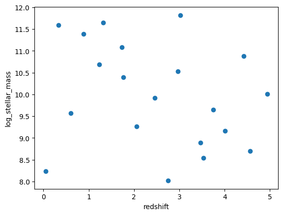
Above we have defined a parameter space with two parameters: redshift and log_stellar_mass. We have defined the ranges for these parameters as (0.0, 5.0) and (8.0, 12.0) respectively. We then use the draw_from_hypercube function to draw 100 samples from this parameter space, which returns a dictionary of arrays containing the values for each parameter.
[3]:
param_grid = draw_from_hypercube(param_ranges, 20, rng=42)
If we plot these values, we can see that the parameter space is sampled more evenly than if we had used random sampling.
[4]:
plt.scatter(param_grid["redshift"], param_grid["log_stellar_mass"])
plt.xlabel("redshift")
plt.ylabel("log_stellar_mass")
[4]:
Text(0, 0.5, 'log_stellar_mass')
For this basic tutorial, we will define a 6 dimensional parameter space four our library of galaxies. We will draw 10,000 samples—a size chosen for quick demonstration, though a real, useful library would require significantly more samples—to construct our synthetic galaxy population.
Our six parameters are:
redshift: The redshift of the galaxylog_stellar_mass: The logarithm (base 10) of the stellar mass in units of solar masslog_zmet: The logarithm (base 10) of the stellar metallicitypeak_age: The age corresponding to the peak of the log-normal star formation history (SFH)tau: The dimensionless width of the log-normal SFHtau_v: The V-band optical depth
[5]:
Ngal = 100

param_dict = {
    "redshift": (0, 5),
    "log_stellar_mass": (8, 12),
    "log_zmet": (-4.0, -1.4),
    "peak_age_norm": (0.0, 0.99),  # fraction of the age of the universe
    "tau": (0.1, 2.0),  # dex
    "tau_v": (0.0, 3.0),  # magnitudes
}

params = draw_from_hypercube(param_dict, Ngal, rng=42)
Generating SFH Distributions
In the previous tutorial we saw how to generate a single SFH class instance representing a Constant star formation history. However, in many cases we may want to generate a library of star formation histories that represent a range of different galaxy types. Whilst this can be done entirely manually, synference provides a convenient helper function to generate a library of star formation histories based on a set of parameters.
[6]:
from synthesizer.parametric import SFH

from synference import generate_sfh_basis
The generate_sfh_basis function is used to generate an array of SFH objects from our sampled parameter arrays.
To do this, we pass the function the desired SFH class (e.g. SFH.LogNormal) and the dictionary of sampled arrays. The function then returns an array of instantiated SFH instances, where the paramaters for each object are drawn from the arrays we provided. We also require that you provide parameter units using unyt Units (e.g. Myr for age), which ensures that the parameters are correctly interpreted by the SFH class.
Optionally, we can define a redshift dependent star formation history. To this, designate a parameter which will be scaled by the available lookback time at the redshift of the galaxy. This is useful for parameters which are physically constrained by the age of the universe, such as the peak age of a log-normal SFH.
[7]:
sfh_models, _ = generate_sfh_basis(
    sfh_type=SFH.LogNormal,
    sfh_param_names=["peak_age_norm", "tau"],
    sfh_param_arrays=[params["peak_age_norm"], params["tau"]],
    sfh_param_units=[None, None],
    redshifts=params["redshift"],
)

print(len(sfh_models), type(sfh_models[0]))
Creating SFHs: 100it [00:00, 887.47it/s]
100 <class 'synthesizer.parametric.sf_hist.LogNormal'>
We can see that the generate_sfh_basis function has returned an array of 1000 SFH.LogNormal instances, each with the parameters drawn from the arrays we provided.
Generating Metallicity Distributions
In the same manner that we can generate a library of star formation histories, we can also generate a library of metallicity histories. While we don’t provide a helper function for this, these are simpler to generate:
[8]:
from synthesizer.parametric import ZDist

zdists = []

for z in params["log_zmet"]:
    zdists.append(ZDist.DeltaConstant(log10metallicity=z))

print(len(zdists), zdists[0])
100 ----------
SUMMARY OF PARAMETERISED METAL ENRICHMENT HISTORY
<class 'synthesizer.parametric.metal_dist.DeltaConstant'>
metallicity: None
log10metallicity: -3.13879132270813
----------
The above code loops over the metallicities drawn from the prior samples. For each metallicity value, it instantiates the metallicity class, and append the result to a list.
Setting up the rest of our Synthesizer model
Grid
We must load in the SPS grid we will use to generate our stellar and nebular spectra. As we will be generating a lot of spectra, we may also wish to set the wavelength array defined for the grid, to limit the resolution and min/max limits to save storage space and processing time. This can be set on creating a Grid by passing a new_lam argument with a new wavelength array, onto which the grid will be interpolated using a flux-conserving interpolation. We have a helper method to generate
a new wavelength array with constant R between two wavelengths.
Here we are using a BPASS SPS grid with a Chabrier 2003 IMF, which has been post-processed with Cloudy 23.01.
[9]:
from synthesizer.grid import Grid
from unyt import Angstrom

from synference import generate_constant_R

new_lam = generate_constant_R(R=300, start=1 * Angstrom, stop=50_000 * Angstrom)

grid = Grid("test_grid", new_lam=new_lam)
Emission Models
If you’ve already read the previous tutorial, you’ll remember that emission models are crucial for defining the process by which we generate observables of our galaxies. The GalaxyBasis class takes a single EmissionModel instance which is used for all galaxy generation.
In this example, as we have defined our model with a dust component (tau_v), we will use a TotalEmission emission model.
[10]:
from synthesizer.emission_models import TotalEmission
from synthesizer.emission_models.attenuation import PowerLaw

emission_model = TotalEmission(
    grid=grid,
    dust_curve=PowerLaw(slope=-0.7),
)

emission_model.plot_emission_tree()
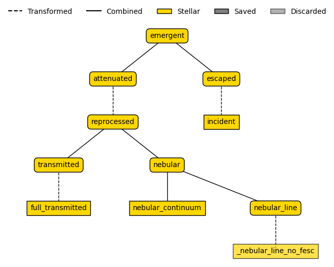
[10]:
(<Figure size 600x600 with 1 Axes>, <Axes: >)
[11]:
emission_model._models["attenuated"].__dict__
[11]:
{'label': 'attenuated',
 '_lam': array([1.00000000e+00, 1.00166667e+00, 1.00333611e+00, ...,
        8.97092337e+05, 8.98587491e+05, 9.00085136e+05], shape=(8234,)),
 'fixed_parameters': {},
 '_emitter': 'stellar',
 '_per_particle': False,
 'masks': [],
 '_lam_mask': None,
 '_is_extracting': False,
 '_is_combining': False,
 '_is_transforming': True,
 '_is_generating': False,
 '_transformer': PowerLaw(slope=-0.7),
 '_apply_to': <synthesizer.emission_models.stellar.models.ReprocessedEmission at 0x7f1d32132590>,
 '_children': {<synthesizer.emission_models.stellar.models.ReprocessedEmission at 0x7f1d32132590>},
 '_parents': {<synthesizer.emission_models.stellar.models.EmergentEmission at 0x7f1e4ced7460>},
 '_scale_by': (),
 '_post_processing': (),
 '_energy_balance_models': None,
 '_scaler_model': None,
 'related_models': {<synthesizer.emission_models.base_model.StellarEmissionModel at 0x7f1d3215f760>},
 '_save': True,
 '_extract_keys': {'nebular_continuum': 'nebular_continuum',
  '_nebular_line_no_fesc': 'linecont',
  'full_transmitted': 'transmitted',
  'incident': 'incident'},
 '_models': {'attenuated': <synthesizer.emission_models.models.AttenuatedEmission at 0x7f1e246e0400>,
  'reprocessed': <synthesizer.emission_models.stellar.models.ReprocessedEmission at 0x7f1d32132590>,
  'nebular': <synthesizer.emission_models.stellar.models.NebularEmission at 0x7f1d32133a90>,
  'nebular_continuum': <synthesizer.emission_models.stellar.models.NebularContinuumEmission at 0x7f1d32132050>,
  'nebular_line': <synthesizer.emission_models.stellar.models.NebularLineEmission at 0x7f1d320ec6d0>,
  '_nebular_line_no_fesc': <synthesizer.emission_models.base_model.StellarEmissionModel at 0x7f1d321321d0>,
  'transmitted': <synthesizer.emission_models.stellar.models.TransmittedEmissionWithEscaped at 0x7f1d3215f6a0>,
  'full_transmitted': <synthesizer.emission_models.base_model.StellarEmissionModel at 0x7f1d3215f5b0>,
  'escaped': <synthesizer.emission_models.base_model.StellarEmissionModel at 0x7f1d3215f760>,
  'incident': <synthesizer.emission_models.stellar.models.IncidentEmission at 0x7f1d320ef6d0>}}
You’ll notice that above, unlike in the first tutorial, we didn’t set the optical depth tau_v directy on the emission model. This is because we want it to vary between galaxies, so we will instead pass this attribute to GalaxyBasis to set it on the individual Galaxy level.
Instruments and Filters
Finally, the last thing we have to define is what we actually want to observe. We could simply call get_spectra to get the rest-frame and observed-frame spectra on the wavelengths of the Grid.
But what if we want observations in specific photometric filters, or matched to the resolution of a specfic spectroscopic instrument? We must create and define an Instrument, which contains this information.
Here we will load a predefined NIRCam instrument containing its wideband photometric filters.
[12]:
from synthesizer.instruments import JWSTNIRCamWide

instrument = JWSTNIRCamWide()
---------------------------------------------------------------------------
TimeoutError                              Traceback (most recent call last)
File /opt/hostedtoolcache/Python/3.10.20/x64/lib/python3.10/urllib/request.py:1348, in AbstractHTTPHandler.do_open(self, http_class, req, **http_conn_args)
   1347 try:
-> 1348     h.request(req.get_method(), req.selector, req.data, headers,
   1349               encode_chunked=req.has_header('Transfer-encoding'))
   1350 except OSError as err: # timeout error

File /opt/hostedtoolcache/Python/3.10.20/x64/lib/python3.10/http/client.py:1303, in HTTPConnection.request(self, method, url, body, headers, encode_chunked)
   1302 """Send a complete request to the server."""
-> 1303 self._send_request(method, url, body, headers, encode_chunked)

File /opt/hostedtoolcache/Python/3.10.20/x64/lib/python3.10/http/client.py:1349, in HTTPConnection._send_request(self, method, url, body, headers, encode_chunked)
   1348     body = _encode(body, 'body')
-> 1349 self.endheaders(body, encode_chunked=encode_chunked)

File /opt/hostedtoolcache/Python/3.10.20/x64/lib/python3.10/http/client.py:1298, in HTTPConnection.endheaders(self, message_body, encode_chunked)
   1297     raise CannotSendHeader()
-> 1298 self._send_output(message_body, encode_chunked=encode_chunked)

File /opt/hostedtoolcache/Python/3.10.20/x64/lib/python3.10/http/client.py:1058, in HTTPConnection._send_output(self, message_body, encode_chunked)
   1057 del self._buffer[:]
-> 1058 self.send(msg)
   1060 if message_body is not None:
   1061
   1062     # create a consistent interface to message_body

File /opt/hostedtoolcache/Python/3.10.20/x64/lib/python3.10/http/client.py:996, in HTTPConnection.send(self, data)
    995 if self.auto_open:
--> 996     self.connect()
    997 else:

File /opt/hostedtoolcache/Python/3.10.20/x64/lib/python3.10/http/client.py:962, in HTTPConnection.connect(self)
    961 sys.audit("http.client.connect", self, self.host, self.port)
--> 962 self.sock = self._create_connection(
    963     (self.host,self.port), self.timeout, self.source_address)
    964 # Might fail in OSs that don't implement TCP_NODELAY

File /opt/hostedtoolcache/Python/3.10.20/x64/lib/python3.10/socket.py:857, in create_connection(address, timeout, source_address)
    856 try:
--> 857     raise err
    858 finally:
    859     # Break explicitly a reference cycle

File /opt/hostedtoolcache/Python/3.10.20/x64/lib/python3.10/socket.py:845, in create_connection(address, timeout, source_address)
    844     sock.bind(source_address)
--> 845 sock.connect(sa)
    846 # Break explicitly a reference cycle

TimeoutError: [Errno 110] Connection timed out

During handling of the above exception, another exception occurred:

URLError                                  Traceback (most recent call last)
File /opt/hostedtoolcache/Python/3.10.20/x64/lib/python3.10/site-packages/synthesizer/instruments/filters.py:2041, in Filter._make_svo_filter(self)
   2040 try:
-> 2041     with urllib.request.urlopen(self.svo_url) as f:
   2042         # Get the root of the XML tree
   2043         root = ElementTree.parse(f).getroot()

File /opt/hostedtoolcache/Python/3.10.20/x64/lib/python3.10/urllib/request.py:216, in urlopen(url, data, timeout, cafile, capath, cadefault, context)
    215     opener = _opener
--> 216 return opener.open(url, data, timeout)

File /opt/hostedtoolcache/Python/3.10.20/x64/lib/python3.10/urllib/request.py:519, in OpenerDirector.open(self, fullurl, data, timeout)
    518 sys.audit('urllib.Request', req.full_url, req.data, req.headers, req.get_method())
--> 519 response = self._open(req, data)
    521 # post-process response

File /opt/hostedtoolcache/Python/3.10.20/x64/lib/python3.10/urllib/request.py:536, in OpenerDirector._open(self, req, data)
    535 protocol = req.type
--> 536 result = self._call_chain(self.handle_open, protocol, protocol +
    537                           '_open', req)
    538 if result:

File /opt/hostedtoolcache/Python/3.10.20/x64/lib/python3.10/urllib/request.py:496, in OpenerDirector._call_chain(self, chain, kind, meth_name, *args)
    495 func = getattr(handler, meth_name)
--> 496 result = func(*args)
    497 if result is not None:

File /opt/hostedtoolcache/Python/3.10.20/x64/lib/python3.10/urllib/request.py:1377, in HTTPHandler.http_open(self, req)
   1376 def http_open(self, req):
-> 1377     return self.do_open(http.client.HTTPConnection, req)

File /opt/hostedtoolcache/Python/3.10.20/x64/lib/python3.10/urllib/request.py:1351, in AbstractHTTPHandler.do_open(self, http_class, req, **http_conn_args)
   1350 except OSError as err: # timeout error
-> 1351     raise URLError(err)
   1352 r = h.getresponse()

URLError: <urlopen error [Errno 110] Connection timed out>

During handling of the above exception, another exception occurred:

SVOInaccessible                           Traceback (most recent call last)
Cell In[12], line 3
      1 from synthesizer.instruments import JWSTNIRCamWide
----> 3 instrument = JWSTNIRCamWide()

File /opt/hostedtoolcache/Python/3.10.20/x64/lib/python3.10/site-packages/synthesizer/instruments/premade.py:333, in JWSTNIRCamWide.__init__(self, label, filter_lams, depth, depth_app_radius, snrs, psfs, noise_maps, filter_subset, **kwargs)
    330 filter_codes = filter_subset or self.available_filters
    332 # Get the filters from SVO
--> 333 filters = FilterCollection(
    334     filter_codes=filter_codes,
    335     new_lam=filter_lams,
    336 )
    338 # Call the parent constructor with the appropriate parameters
    339 # NIRCam
    340 PhotometricImager.__init__(
    341     self,
    342     label=label,
   (...)
    350     **kwargs,
    351 )

File /opt/hostedtoolcache/Python/3.10.20/x64/lib/python3.10/site-packages/synthesizer/utils/operation_timers.py:98, in timed.<locals>.decorator.<locals>.wrapped(*args, **kwargs)
     94 tic(timer_name)
     95 try:
     96     # Return the wrapped function result unchanged so the decorator
     97     # is transparent aside from its timing side effect.
---> 98     return func(*args, **kwargs)
     99 finally:
    100     # Always stop the timer, even if the wrapped function raises,
    101     # so the timing stack remains balanced.
    102     toc(timer_name)

File /opt/hostedtoolcache/Python/3.10.20/x64/lib/python3.10/site-packages/synthesizer/instruments/filters.py:297, in FilterCollection.__init__(self, filter_codes, tophat_dict, generic_dict, filters, path, new_lam, fill_gaps, verbose)
    295 # Let's make the filters
    296 if filter_codes is not None:
--> 297     self._include_svo_filters(filter_codes)
    298 if tophat_dict is not None:
    299     self._include_top_hat_filters(tophat_dict)

File /opt/hostedtoolcache/Python/3.10.20/x64/lib/python3.10/site-packages/synthesizer/instruments/filters.py:474, in FilterCollection._include_svo_filters(self, filter_codes)
    471 # Loop over the given filter codes
    472 for f in filter_codes:
    473     # Get filter from SVO
--> 474     _filter = Filter(f, new_lam=self.lam)
    476     # Store the filter and its code
    477     self.filters[_filter.filter_code] = _filter

File /opt/hostedtoolcache/Python/3.10.20/x64/lib/python3.10/site-packages/synthesizer/units.py:909, in accepts.<locals>.check_accepts.<locals>.wrapped(*args, **kwargs)
    906 finally:
    907     toc(f"accepts({func.__qualname__})")
--> 909 return func(*bound.args, **bound.kwargs)

File /opt/hostedtoolcache/Python/3.10.20/x64/lib/python3.10/site-packages/synthesizer/utils/operation_timers.py:98, in timed.<locals>.decorator.<locals>.wrapped(*args, **kwargs)
     94 tic(timer_name)
     95 try:
     96     # Return the wrapped function result unchanged so the decorator
     97     # is transparent aside from its timing side effect.
---> 98     return func(*args, **kwargs)
     99 finally:
    100     # Always stop the timer, even if the wrapped function raises,
    101     # so the timing stack remains balanced.
    102     toc(timer_name)

File /opt/hostedtoolcache/Python/3.10.20/x64/lib/python3.10/site-packages/synthesizer/instruments/filters.py:1770, in Filter.__init__(self, filter_code, transmission, lam_min, lam_max, lam_eff, lam_fwhm, new_lam, hdf)
   1768 # Is this an SVO filter?
   1769 elif "/" in filter_code and "." in filter_code:
-> 1770     self._make_svo_filter()
   1772 # Otherwise we haven't got a valid combination of inputs.
   1773 else:
   1774     raise exceptions.InconsistentArguments(
   1775         "Invalid combination of filter inputs. \n For a generic "
   1776         "filter provide a transmission and wavelength array. "
   (...)
   1781         "wavelength or an effective wavelength and FWHM."
   1782     )

File /opt/hostedtoolcache/Python/3.10.20/x64/lib/python3.10/site-packages/synthesizer/instruments/filters.py:2052, in Filter._make_svo_filter(self)
   2049         data = root.find(".//TABLEDATA")
   2051 except URLError:
-> 2052     raise exceptions.SVOInaccessible(
   2053         (
   2054             f"The SVO Database at {self.svo_url} "
   2055             "is not responding. Is it down?"
   2056         )
   2057     )
   2059 # Throw an error if we didn't find the filter.
   2060 if field is None:

SVOInaccessible: The SVO Database at http://svo2.cab.inta-csic.es/theory/fps/fps.php?ID=JWST/NIRCam.F070W is not responding. Is it down?
Putting it all together - Generating our Library
Now that we have all the constituent components of our model we can finally put it all together and generate our library of observables. Firstly we simply instantiate a GalaxyBasis object, passing in the various components we have created above.
We must also define a galaxy_params dictionary, which contains any arguments we wish to set on the individual Galaxy objects, rather than globally on the emission model.
In this case, we set the V-band optical depth (tau_v) for each galaxy. However, this dictionary can include any number of emission model parameters intended to vary per galaxy, star or black hole instance.
We are also explicitly telling the code to ignore the max_age parameter. While max_age varies per galaxy, it is redundant because it is already a defined transformation of the redshift, meaning its value can be calculated from another parameter already present in our set.
We give this model a name, ‘testing_model’, which will be used when saving the output files.
[13]:
galaxy_params = {"tau_v": params["tau_v"]}

galaxy_basis = GalaxyBasis(
    grid=grid,
    model_name="testing_model",
    redshifts=params["redshift"],
    emission_model=emission_model,
    instrument=instrument,
    sfhs=sfh_models,
    metal_dists=zdists,
    log_stellar_masses=params["log_stellar_mass"],
    galaxy_params=galaxy_params,
    params_to_ignore=["max_age"],
)
---------------------------------------------------------------------------
NameError                                 Traceback (most recent call last)
Cell In[13], line 8
      1 galaxy_params = {"tau_v": params["tau_v"]}
      3 galaxy_basis = GalaxyBasis(
      4     grid=grid,
      5     model_name="testing_model",
      6     redshifts=params["redshift"],
      7     emission_model=emission_model,
----> 8     instrument=instrument,
      9     sfhs=sfh_models,
     10     metal_dists=zdists,
     11     log_stellar_masses=params["log_stellar_mass"],
     12     galaxy_params=galaxy_params,
     13     params_to_ignore=["max_age"],
     14 )

NameError: name 'instrument' is not defined
Now that we have created an instance of the GalaxyBasis, we can run the library creation using the create_mock_library method. Here we set the output model name, which emission model key to generate the library from (by default total), as well as setting optional configuration parameters. We can see for our above emission model that the root key is emergent, so we will set that here. We could also change the output folder, which will otherwise default to the internal ‘libraries/’
folder where the synference code is installed.
The create_mock_library method utilizes Synthesizer’s built-in Pipeline functionality, which handles processing the galaxies in batches and supports parallel execution if Synthesizer has been installed with OpenMP support (see the Synthesizer installation documentation for more information). This significantly speeds up galaxy library creation, making it scalable across cores and nodes for generating very large samples.
We also save the max_age parameter, which is a derived parameter based on the redshift of the galaxy. This is useful for later analysis so we can easily reconstruct the original parameter space.
[14]:
def max_age(x):
    """Compute the maximum age of the universe at a given redshift."""
    from astropy.cosmology import Planck18 as cosmo
    from unyt import Myr

    return cosmo.age(x["redshift"]).to_value("Myr") * Myr


param_transforms = {"max_age": ("max_age", max_age)}
[15]:
galaxy_basis.create_mock_library(
    "test_model_library",
    emission_model_key="emergent",
    overwrite=True,
    parameter_transforms_to_save=param_transforms,
    n_proc=1,
)
---------------------------------------------------------------------------
NameError                                 Traceback (most recent call last)
Cell In[15], line 1
----> 1 galaxy_basis.create_mock_library(
      2     "test_model_library",
      3     emission_model_key="emergent",
      4     overwrite=True,
      5     parameter_transforms_to_save=param_transforms,
      6     n_proc=1,
      7 )

NameError: name 'galaxy_basis' is not defined
The above code created a lot of output, but we can break it down. In order, it:
Created the individual galaxies, setting the attributes as we described.
Instantiated a
Pipelineand passed in the array of galaxies.Ran the pipeline for the galaxies to generate the observed spectroscopy and photometry, which is stored in a HDF5 file.
Loaded the saved HDF5 file, extracted the photometry for our emission key ‘emergent’, and generated the photometry and input parameter libraries.
Saved these separate libraries into a different HDF5 file, which will be used by the code later.
Inspecting our Library
There are numerous packages for inspecting HDF5 files, including the h5py package, which you have installed if you have run the code to this point without crashing. For more visual views, we recommend H5Web, which has a VS Code extension, or the command line interface h5forest, which you can find on Github here.
Below we use the h5py library to inspect the structure and contents of our saved dataset:
[16]:
import h5py

from synference import library_folder

with h5py.File(f"{library_folder}/test_model_library.hdf5") as f:
    for dataset in f:
        print(f"- {dataset}")
        for array in f[dataset]:
            print(f"    - {array}")
            if isinstance(f[dataset][array], h5py.Dataset):
                print(f"        - Dataset shape: {f[dataset][array].shape}")
            elif isinstance(f[dataset][array], h5py.Group):
                print(f"        - Group: {list(f[dataset][array].keys())}")
---------------------------------------------------------------------------
FileNotFoundError                         Traceback (most recent call last)
Cell In[16], line 5
      1 import h5py
      3 from synference import library_folder
----> 5 with h5py.File(f"{library_folder}/test_model_library.hdf5") as f:
      6     for dataset in f:
      7         print(f"- {dataset}")

File /opt/hostedtoolcache/Python/3.10.20/x64/lib/python3.10/site-packages/h5py/_hl/files.py:555, in File.__init__(self, name, mode, driver, libver, userblock_size, swmr, rdcc_nslots, rdcc_nbytes, rdcc_w0, track_order, fs_strategy, fs_persist, fs_threshold, fs_page_size, page_buf_size, min_meta_keep, min_raw_keep, locking, alignment_threshold, alignment_interval, meta_block_size, track_times, **kwds)
    546     fapl = make_fapl(driver, libver, rdcc_nslots, rdcc_nbytes, rdcc_w0,
    547                      locking, page_buf_size, min_meta_keep, min_raw_keep,
    548                      alignment_threshold=alignment_threshold,
    549                      alignment_interval=alignment_interval,
    550                      meta_block_size=meta_block_size,
    551                      **kwds)
    552     fcpl = make_fcpl(track_order=track_order, track_times=track_times,
    553                      fs_strategy=fs_strategy, fs_persist=fs_persist,
    554                      fs_threshold=fs_threshold, fs_page_size=fs_page_size)
--> 555     fid = make_fid(name, mode, userblock_size, fapl, fcpl, swmr=swmr)
    557 if isinstance(libver, tuple):
    558     self._libver = libver

File /opt/hostedtoolcache/Python/3.10.20/x64/lib/python3.10/site-packages/h5py/_hl/files.py:232, in make_fid(name, mode, userblock_size, fapl, fcpl, swmr)
    230     if swmr:
    231         flags |= h5f.ACC_SWMR_READ
--> 232     fid = h5f.open(name, flags, fapl=fapl)
    233 elif mode == 'r+':
    234     fid = h5f.open(name, h5f.ACC_RDWR, fapl=fapl)

File h5py/_objects.pyx:54, in h5py._objects.with_phil.wrapper()

File h5py/_objects.pyx:55, in h5py._objects.with_phil.wrapper()

File h5py/h5f.pyx:106, in h5py.h5f.open()

FileNotFoundError: [Errno 2] Unable to synchronously open file (unable to open file: name = '/opt/hostedtoolcache/Python/3.10.20/x64/lib/python3.10/libraries/test_model_library.hdf5', errno = 2, error message = 'No such file or directory', flags = 0, o_flags = 0)
Our HDF5 file contains the following key components:
Parameters array: Contains the input samples for all 6 parameters we defined for our prior (mass, redshift, tau_v, metallicity, peak_age, tau) with 100 draws from the prior for each parameter
Photometry array: Our synthetic observables consisting of 8 photometric fluxes (corresponding to the 8 NIRCam widebands) calculated for each of the 100 galaxy draws
Supplementary parameters array: An empty supplementary parameters array in this case, designed to store optional derived quantities such as star formation rates, or the surviving stellar mass
Model Group: This stores information about the emission model and instrument used, allowing us recreate the emission model and instrument later if we need to
It’s worth noting that the only required arrays are the ‘parameters’ and ‘photometry’ datasets. So you can entirely avoid using Synthesizer and build models externally using your code and method of choice, as long as you can produde a HDF5 array with the same simple format you will be able to use the SBI functionality of Synference with your code. Please see this example, where we train a model from the outputs of the hydrodynamical simulation SPHINX.
Plotting a galaxy from our model
Synference has some debug methods to plot specific or random individual galaxy SEDs, photometry and star formation histories - plot_galaxy and plot_random_galaxy. Below we plot a random galaxy from the model.
[17]:
galaxy_basis.plot_random_galaxy(masses=params["log_stellar_mass"], emission_model_keys=["emergent"])
---------------------------------------------------------------------------
NameError                                 Traceback (most recent call last)
Cell In[17], line 1
----> 1 galaxy_basis.plot_random_galaxy(masses=params["log_stellar_mass"], emission_model_keys=["emergent"])

NameError: name 'galaxy_basis' is not defined