Basic SBI Model Training¶

In this tutorial, we will walk through the process of training a simulation-based inference (SBI) model using the synference package. We will assume we already have a library of simulations and corresponding parameters.

First let’s consider the training process more generally. The main steps involved in training an SBI model are:

Prepare the Simulation Data: Gather a set of simulations and their corresponding parameters.
Choose a Model Architecture: Select an appropriate neural network architecture for the SBI model.
Define the Training Procedure: Set up the training loop, loss function, and optimization algorithm.
Train the Model: Run the training process and monitor performance.
Evaluate the Model: Assess the trained model’s performance on a validation set.

Now let’s look at how to implement these steps using synference.

[1]:

from synference import SBI_Fitter, test_data_dir

/opt/hostedtoolcache/Python/3.10.19/x64/lib/python3.10/site-packages/tqdm/auto.py:21: TqdmWarning: IProgress not found. Please update jupyter and ipywidgets. See https://ipywidgets.readthedocs.io/en/stable/user_install.html
  from .autonotebook import tqdm as notebook_tqdm

From the output of the library generation tutorials, we should have a HDF5 file called test_model_library.hdf5 in our ‘libraries/’ directory. If you don’t have this file, please refer to the Library Generation tutorial.

We can directly use this file to instantiate a SBI_Fitter instance, which is the class which handles training and evaluating SBI models in synference.

[2]:

fitter = SBI_Fitter.init_from_hdf5(
    model_name="test", hdf5_path=f"{test_data_dir}/example_model_library.hdf5"
)

Feature and Parameter Arrays¶

Now this fitter has loaded the generated observations and parameters from the HDF5 file. Note that the data is not yet normalized or set up with the correct features for training. We will handle that in the next steps.

We can see the names of the observations.

[3]:

print(fitter.raw_observation_names)

['JWST/NIRCam.F070W' 'JWST/NIRCam.F090W' 'JWST/NIRCam.F115W'
 'JWST/NIRCam.F150W' 'JWST/NIRCam.F200W' 'JWST/NIRCam.F277W'
 'JWST/NIRCam.F356W' 'JWST/NIRCam.F444W']

The names of the features:

[4]:

print(fitter.parameter_names)

['redshift' 'log_mass' 'tau_v' 'tau' 'peak_age' 'log10metallicity']

and any associated parameters units:

[5]:

print(fitter.parameter_units)

['dimensionless' 'log10_Msun' 'mag' 'dimensionless' 'Myr' 'log10(Zmet)']

The actual array itself is stored in the parameter_array attribute, which we will just print the first 10 entries of here:

[6]:

print(fitter.parameter_array[:10])

[[ 2.05416274e+00  1.04035606e+01  1.22474718e+00  9.36861515e-01
   1.69158648e+03 -3.13879132e+00]
 [ 2.00016856e+00  1.04899187e+01  1.28473628e+00  1.60899329e+00
   3.02503141e+03 -3.87390995e+00]
 [ 2.18753195e+00  1.15228844e+01  2.18956232e+00  1.20334947e+00
   1.86831172e+03 -3.46571136e+00]
 [ 2.11274648e+00  9.81967258e+00  5.74459910e-01  8.06611896e-01
   2.01560364e+03 -1.89818966e+00]
 [ 2.44652700e+00  9.17687321e+00  1.38670945e+00  1.77724314e+00
   3.07231417e+02 -2.88550878e+00]
 [ 6.84367716e-01  1.14148254e+01  2.61994505e+00  3.89508367e-01
   3.59630292e+03 -1.86997616e+00]
 [ 1.49105906e-01  1.00042429e+01  1.95352912e+00  1.27394879e+00
   1.13156527e+04 -2.40571117e+00]
 [ 1.71895242e+00  1.17945662e+01  1.94888246e+00  2.07960412e-01
   1.57720040e+03 -3.86293936e+00]
 [ 2.84610391e+00  9.41966534e+00  2.85131145e+00  8.91395509e-01
   1.19775692e+03 -3.77944398e+00]
 [ 2.45635724e+00  1.03770952e+01  1.80910027e+00  2.73230791e-01
   2.36855774e+03 -1.71073520e+00]]

And a similar logic for the observations:

[7]:

print(fitter.raw_observation_grid[:, :10])

[[1.55361035e+02 6.62787615e+01 2.93631144e+02 6.01755184e+01
  6.08683670e+00 2.52897265e+03 6.31139334e+03 5.55954909e+02
  3.01451722e-01 7.46139935e-02]
 [2.40530441e+02 1.13258320e+02 5.88940061e+02 7.87135295e+01
  9.31069105e+00 6.79137932e+03 1.07562514e+04 1.35413814e+03
  7.49976727e-01 5.30070034e-01]
 [5.07742016e+02 2.91263414e+02 1.41441540e+03 1.44744857e+02
  1.48766062e+01 1.40988387e+04 1.63680472e+04 5.82525117e+03
  1.77367012e+00 5.52317547e+00]
 [1.06025886e+03 5.80749330e+02 3.79225364e+03 3.03962040e+02
  3.73309422e+01 2.65854161e+04 2.33425604e+04 1.08011228e+04
  5.90461870e+00 3.40313785e+01]
 [1.49439723e+03 8.83105895e+02 6.47315587e+03 4.27806729e+02
  5.66841099e+01 4.68630971e+04 3.13794258e+04 1.76892096e+04
  1.37485025e+01 1.01136398e+02]
 [1.90476605e+03 1.16731581e+03 9.31606212e+03 6.26340520e+02
  8.70344677e+01 8.13157865e+04 2.26920392e+04 2.70938604e+04
  2.74803669e+01 2.37788360e+02]
 [2.36584297e+03 1.41584377e+03 1.28469681e+04 8.12406290e+02
  1.16919381e+02 7.99288041e+04 1.74361191e+04 3.40880141e+04
  3.78438853e+01 3.99970276e+02]
 [2.70394000e+03 1.58965237e+03 1.54602400e+04 9.96181433e+02
  1.33611502e+02 5.93842217e+04 1.33736683e+04 4.01845570e+04
  5.17631635e+01 5.66103013e+02]]

The first step is to turn this raw library of photometric observations into a set of features that can be used for training. This is done with the fitter.create_feature_array method.

This method handles the following tasks:

Normalizing the observations (e.g., converting magnitudes to fluxes, normalizing by a reference band, etc.)
Creating features from the observations (e.g., colors, ratios, etc.)
Removing photometric bands in the library from the feature array that are not present in the observations.
Handling missing data (e.g., setting features to NaN if any of the required bands are missing)
Adding additional features (e.g., redshift) from the parameter array to the feature array.
Adding realistic noise to the features based on a provided noise model (see the Noise Models tutorial for more details).
Adding photometric uncertainties to the feature array.

The default configuration of this method doesn’t do all of these however. By default, all photometric bands are kept, no additional features are added, and no noise is added. The default normalization is to convert the raw array of photometry to AB magnitudes only.

We call the method below and we can see it prints information about the features it creates.

[8]:

fitter.create_feature_array();

2025-11-13 20:07:32,526 | synference | INFO     | ---------------------------------------------
2025-11-13 20:07:32,527 | synference | INFO     | Features: 8 features over 100 samples
2025-11-13 20:07:32,527 | synference | INFO     | ---------------------------------------------
2025-11-13 20:07:32,528 | synference | INFO     | Feature: Min - Max
2025-11-13 20:07:32,529 | synference | INFO     | ---------------------------------------------
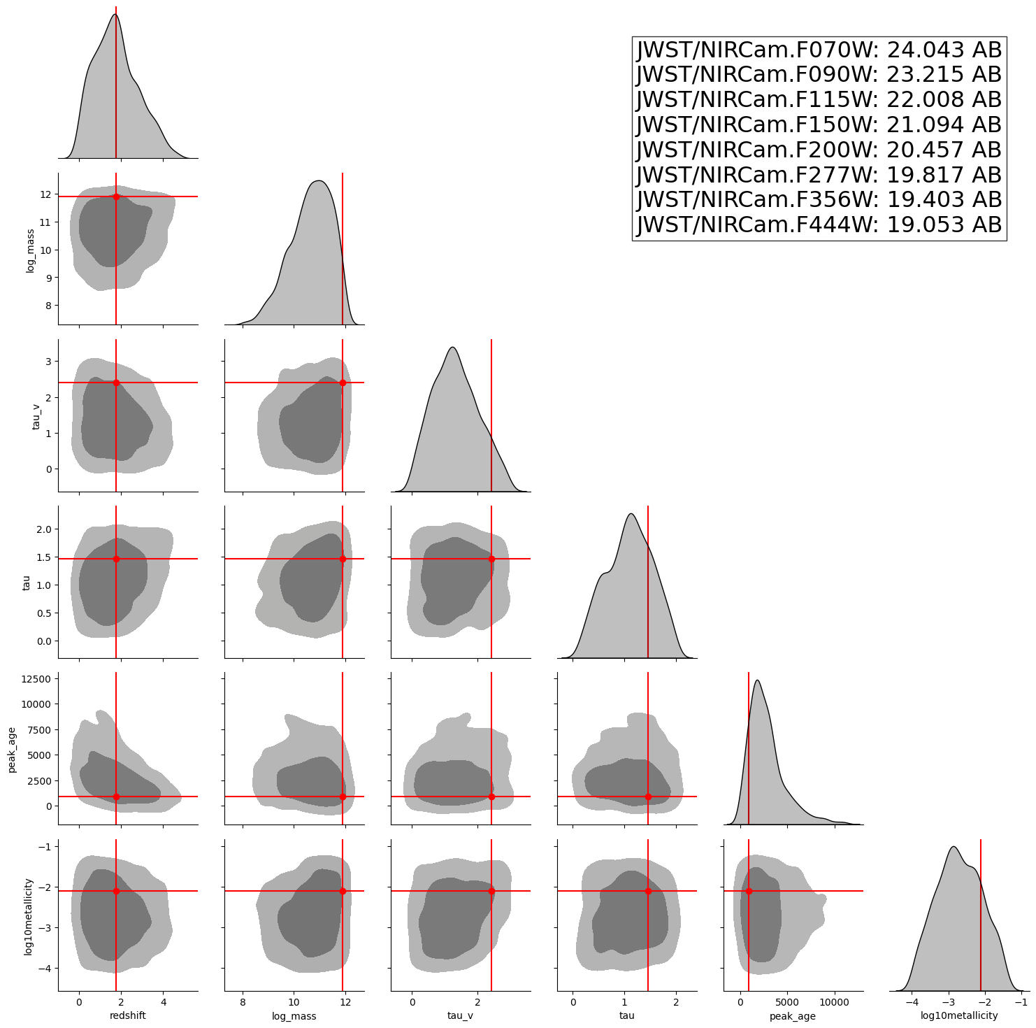
2025-11-13 20:07:32,530 | synference | INFO     | JWST/NIRCam.F070W: 7.131974 - 42.758 AB
2025-11-13 20:07:32,531 | synference | INFO     | JWST/NIRCam.F090W: 7.108530 - 39.933 AB
2025-11-13 20:07:32,532 | synference | INFO     | JWST/NIRCam.F115W: 7.012560 - 38.354 AB
2025-11-13 20:07:32,532 | synference | INFO     | JWST/NIRCam.F150W: 6.969396 - 36.997 AB
2025-11-13 20:07:32,533 | synference | INFO     | JWST/NIRCam.F200W: 7.133157 - 35.470 AB
2025-11-13 20:07:32,534 | synference | INFO     | JWST/NIRCam.F277W: 7.670149 - 33.243 AB
2025-11-13 20:07:32,534 | synference | INFO     | JWST/NIRCam.F356W: 8.072730 - 32.490 AB
2025-11-13 20:07:32,536 | synference | INFO     | JWST/NIRCam.F444W: 8.353975 - 31.965 AB
2025-11-13 20:07:32,537 | synference | INFO     | ---------------------------------------------

We will proceed with the default configuration for now. More advanced configurations will be covered in later tutorials. Using different normalizations/units or adding additional features can have a significant impact on the performance of the trained SBI model.

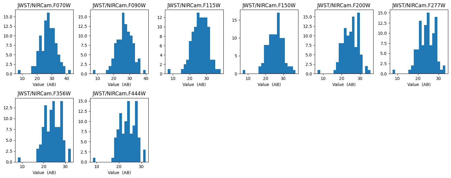
Before we do any fitting, we can inspect the feature and parameter arrays to see the distribution of the data.

Firstly we can look at the feature array, and see the distribution of the photometry given our model and feature array configuration. The below figure shows a histogram of each feature in the feature array.

[9]:

fitter.plot_histogram_feature_array(bins=20);

2025-11-13 20:07:32,953 | synference | INFO     | saving /opt/hostedtoolcache/Python/3.10.19/x64/lib/python3.10/models/test/plots//feature_histogram.png

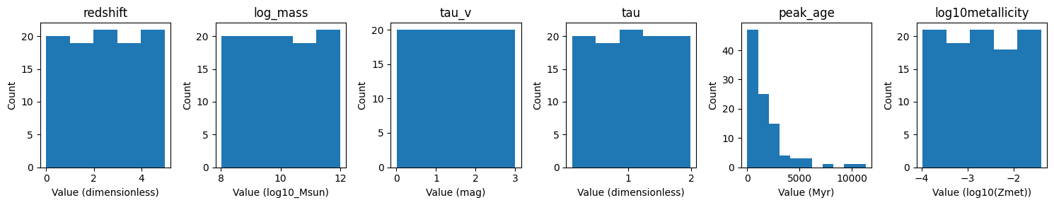
../_images/sbi_train_basic_sbi_model_19_1.png

Secondly we can look at the parameter array, and see the distribution of the parameters given our model and parameter configuration. The below figure shows a histogram of each parameter in the parameter array. We can see that the parameters are uniformly distributed, as expected from our library generation configuration.

[10]:

fitter.plot_histogram_parameter_array();

2025-11-13 20:07:34,461 | synference | INFO     | saving /opt/hostedtoolcache/Python/3.10.19/x64/lib/python3.10/models/test/plots//param_histogram.png

../_images/sbi_train_basic_sbi_model_21_1.png

Training an SBI Model¶

SBI model training is handled with the fitter.train_single_sbi method. This method handles the following tasks:

Creating a prior from the parameter array.
Setting up the neural density estimator (NDE) for the SBI model.
Training the SBI model.
Saving the trained model to disk.
Plotting diagnostics of the trained model.

We will cover the various options for different SBI configurations in later tutorials. For now, we will proceed with the default configuration.

synference is built on top of the LtU-ILI package, which utilizes sbi and lampe for the underlying SBI functionality. The default NDE is a Masked Autoregressive Flow (MAF) from the sbi package. The default prior proposal is a uniform prior over the range of the parameters in the parameter array.

The primary arguments to the fitter.train_single_sbi method are:

train_test_fraction: The fraction of the data to use for training. The rest is used for validation. The default is 0.8.
validation_fraction: The fraction of the training data to use for validation during training. The default is 0.2.
backend: The backend to use for training. Either sbi or lampe. The default is sbi.
hidden_features: The number of hidden features in the NDE. The default is 50.
num_components/transforms: The number of components or transforms in the NDE. The default is 4.
training_batch_size: The batch size for training. The default is 64.
stop_after_epochs: The number of epochs with no improvement to stop training. The default is 15.

There are other methods to turn on or off plotting, model saving, validation, etc. See the docstring for more details.

Now we will run the training, and quite a lot of things will be printed. We are setting name_append to ‘test_1’ so that the trained model is saved with a unique name. If left as the default a timestamp will be used.

[11]:

posterior_model, stats = fitter.run_single_sbi(
    name_append="test_1", random_seed=42, hidden_features=256, num_components=64
)

2025-11-13 20:07:35,225 | synference | INFO     | Splitting dataset with 100 samples into trainingand testing sets with 0.80 train fraction.
2025-11-13 20:07:35,227 | synference | INFO     | ---------------------------------------------
2025-11-13 20:07:35,227 | synference | INFO     | Prior ranges:
2025-11-13 20:07:35,228 | synference | INFO     | ---------------------------------------------
2025-11-13 20:07:35,228 | synference | INFO     | redshift: 0.00 - 4.98 [dimensionless]
2025-11-13 20:07:35,229 | synference | INFO     | log_mass: 8.01 - 11.99 [log10_Msun]
2025-11-13 20:07:35,230 | synference | INFO     | tau_v: 0.01 - 3.00 [mag]
2025-11-13 20:07:35,230 | synference | INFO     | tau: 0.11 - 1.98 [dimensionless]
2025-11-13 20:07:35,231 | synference | INFO     | peak_age: 9.03 - 11315.65 [Myr]
2025-11-13 20:07:35,231 | synference | INFO     | log10metallicity: -3.98 - -1.41 [log10(Zmet)]
2025-11-13 20:07:35,232 | synference | INFO     | ---------------------------------------------
2025-11-13 20:07:35,234 | synference | INFO     | Processing prior...
2025-11-13 20:07:35,237 | synference | INFO     | Creating mdn network with NPE engine and sbi backend.
2025-11-13 20:07:35,238 | synference | INFO     |      hidden_features: 256
2025-11-13 20:07:35,238 | synference | INFO     |      num_components: 64
2025-11-13 20:07:35,239 | synference | INFO     | Training on cpu.

INFO:root:MODEL INFERENCE CLASS: NPE
INFO:root:Training model 1 / 1.

 Neural network successfully converged after 92 epochs.

INFO:root:It took 2.4738616943359375 seconds to train models.
INFO:root:Saving model to /opt/hostedtoolcache/Python/3.10.19/x64/lib/python3.10/models/test

2025-11-13 20:07:37,728 | synference | INFO     | Time to train model(s): 0:00:02.502806
2025-11-13 20:07:37,737 | synference | INFO     | Saved model parameters to /opt/hostedtoolcache/Python/3.10.19/x64/lib/python3.10/models/test/test_test_1_params.pkl.
2025-11-13 20:07:37,876 | synference | INFO     | [ 5.59471250e-01  1.16237526e+01  2.68136740e-01  1.74207807e+00
  9.19759094e+02 -3.81416941e+00]

1385it [00:00, 270884.17it/s]
INFO:root:Saving single posterior plot to /opt/hostedtoolcache/Python/3.10.19/x64/lib/python3.10/models/test/plots/test_1/test_18_plot_single_posterior.jpg...

2025-11-13 20:07:46,830 | synference | INFO     | shapes: X:(20, 8), y:(20, 6)

100%|██████████| 20/20 [00:00<00:00, 295.29it/s]
INFO:root:Saving posterior samples to /opt/hostedtoolcache/Python/3.10.19/x64/lib/python3.10/models/test/plots/test_1/posterior_samples.npy...
INFO:root:Saving coverage plot to /opt/hostedtoolcache/Python/3.10.19/x64/lib/python3.10/models/test/plots/test_1/plot_coverage.jpg...
INFO:root:Saving ranks histogram to /opt/hostedtoolcache/Python/3.10.19/x64/lib/python3.10/models/test/plots/test_1/ranks_histogram.jpg...
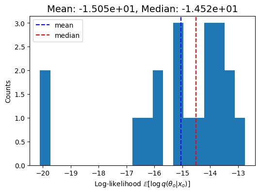
INFO:root:Mean logprob: -1.4675e+01Median logprob: -1.3933e+01
INFO:root:Saving true logprobs to /opt/hostedtoolcache/Python/3.10.19/x64/lib/python3.10/models/test/plots/test_1/true_logprobs.npy...
INFO:root:Saving true logprobs plot to /opt/hostedtoolcache/Python/3.10.19/x64/lib/python3.10/models/test/plots/test_1/plot_true_logprobs.jpg...
INFO:matplotlib.mathtext:Substituting symbol E from STIXNonUnicode
100%|██████████| 100/100 [00:00<00:00, 721.86it/s]

2025-11-13 20:07:48,500 | synference | INFO     | Evaluating model...
2025-11-13 20:07:48,501 | synference | WARNING  | Transposing samples to match shape (num_objects, num_samples, num_parameters).

100%|██████████| 200/200 [00:00<00:00, 749.75it/s]
Log prob: 100%|██████████| 20/20 [00:00<00:00, 108.20it/s]

2025-11-13 20:07:48,962 | synference | INFO     | ============================================================
2025-11-13 20:07:48,963 | synference | INFO     | MODEL PERFORMANCE METRICS
2025-11-13 20:07:48,964 | synference | INFO     | ============================================================
2025-11-13 20:07:48,964 | synference | INFO     | Full Model Metrics:
2025-11-13 20:07:48,965 | synference | INFO     | ----------------------------------------
2025-11-13 20:07:48,965 | synference | INFO     | TARP..................... 0.121250
2025-11-13 20:07:48,967 | synference | INFO     | LOG DPIT MAX............. 0.564099
2025-11-13 20:07:48,968 | synference | INFO     | MEAN LOG PROB............ -14.522387
2025-11-13 20:07:48,968 | synference | INFO     | Parameter-Specific Metrics:
2025-11-13 20:07:48,968 | synference | INFO     | ----------------------------------------
2025-11-13 20:07:48,969 | synference | INFO     | Metric        redshift  log_mass     tau_v       tau        peak_age  log10metallicity
2025-11-13 20:07:48,970 | synference | INFO     | --------------------------------------------------------------------------------------
2025-11-13 20:07:48,970 | synference | INFO     | MSE           1.656271  0.663972  0.569712  0.335677  2652622.516210          0.620463
2025-11-13 20:07:48,971 | synference | INFO     | RMSE          1.286962  0.814845  0.754793  0.579376     1628.687360          0.787695
2025-11-13 20:07:48,973 | synference | INFO     | MEAN AE       0.981742  0.711569  0.643150  0.489777     1465.344738          0.689395
2025-11-13 20:07:48,973 | synference | INFO     | MEDIAN AE     0.762367  0.690642  0.636066  0.439822     1370.900391          0.744325

2025-11-13 20:07:48,974 | synference | INFO     | R SQUARED     0.999957  0.999981  0.999985  0.999991       -0.161590          0.999985
2025-11-13 20:07:48,975 | synference | INFO     | RMSE NORM     0.002003  0.001268  0.001175  0.000902        2.535384          0.001226
2025-11-13 20:07:48,975 | synference | INFO     | MEAN AE NORM  0.001528  0.001108  0.001001  0.000762        2.281108          0.001073
2025-11-13 20:07:48,976 | synference | INFO     | ============================================================

../_images/sbi_train_basic_sbi_model_24_13.png

../_images/sbi_train_basic_sbi_model_24_14.png

../_images/sbi_train_basic_sbi_model_24_15.png

../_images/sbi_train_basic_sbi_model_24_16.png

../_images/sbi_train_basic_sbi_model_24_17.png

INFO:matplotlib.mathtext:Substituting symbol E from STIXNonUnicode

../_images/sbi_train_basic_sbi_model_24_19.png

../_images/sbi_train_basic_sbi_model_24_20.png

The first part of the output shows we split the training data into the training and testing splits, then we create the prior from the parameter library, and show the ranges of each parameter.

The next part shows us creating the neural density estimator (NDE) model, which is a mixture density network (MDN) with 4 components. The model is created using the sbi package, which is built on top of PyTorch.

Then the actual training happens - we see the training epochs increment until the model has stopped improving on the validation set. The training stops after 15 epochs with no improvement, as we set stop_after_epochs=15.

The model is pickled and saved to the output directory for this model, which is models/test_model/ by default. The summary of the training model is saved as a .json file in the same directory. And the configuration of the fitter is also pickled and saved to the same directory, which saves the feature and parameter configuration used for training. A model can be re-loaded later using the fitter.load_model_from_pkl method. We can save in a different format by changing the save_method argument to e.g. torch or hickle.

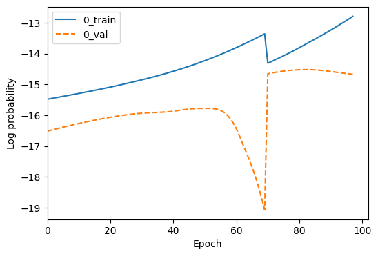
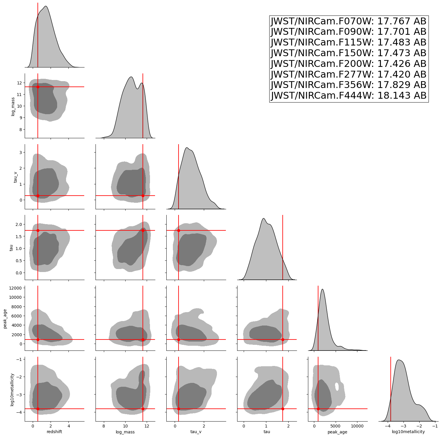
Now we have a trained model. The validation metrics run which include:

A posterior corner plot for a random observation from the test set.
A loss plot which shows the training and validation loss over epochs.
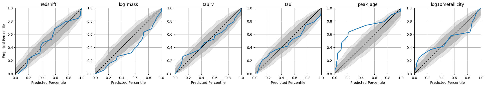
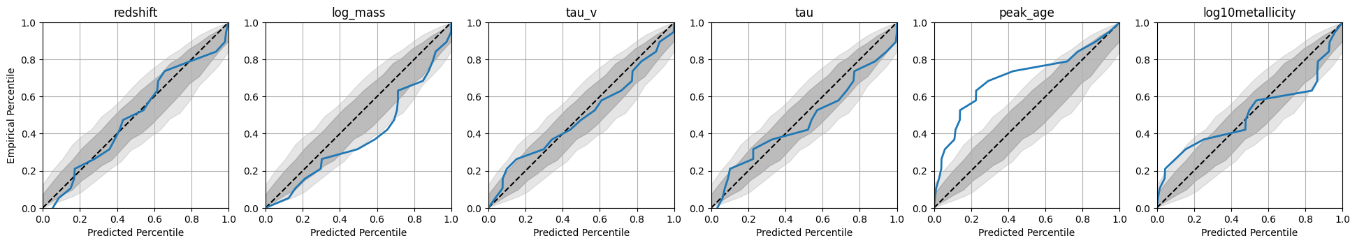
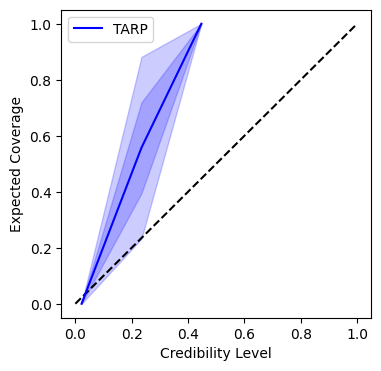
A coverage plot which shows how well the credible intervals of the posterior match the true parameters.
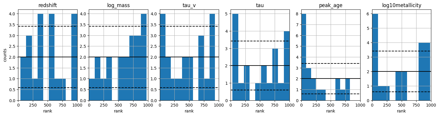
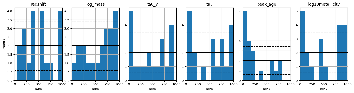
A ranks histogram which shows how well the posterior samples match the true parameters.
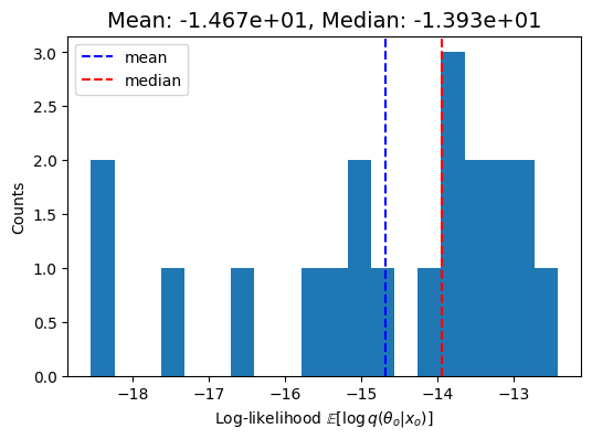
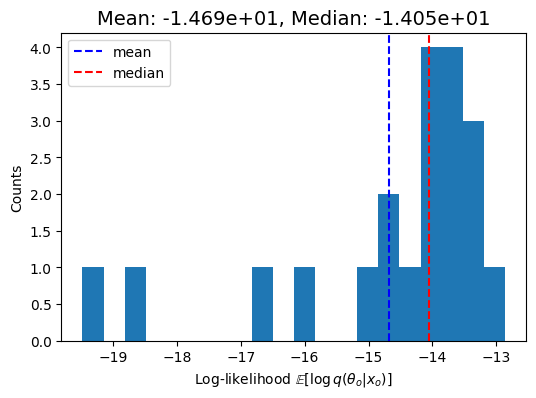
A log_probabiity plot which shows the log probability of the true parameters under the posterior.
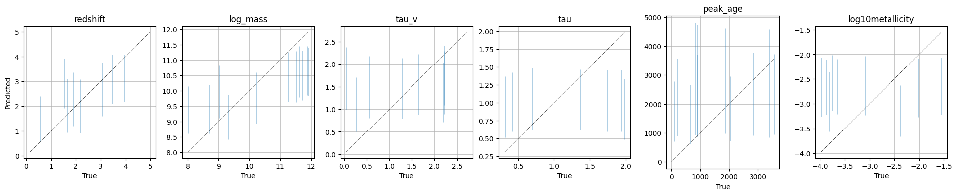
A True vs predicted plot which shows the true parameters vs the maximum a posteriori (MAP) estimate from the posterior.

These plots are shown in the output, and also saved to the plots/ directory in the output folder for this model.

Loading a Trained Model¶

We can load a trained model into an exisiting SBI_Fitter instance using the fitter.load_model_from_pkl method. This method takes the path to the pickled model file as an argument.

If only one model is present in the directory, we can simply provide the directory path and the method will find the model file automatically. If multiple models are present, we can provide the full path to the model file.

[12]:

fitter.load_model_from_pkl("test/test_test_1_posterior.pkl");

2025-11-13 20:07:51,737 | synference | INFO     | Loaded model from /opt/hostedtoolcache/Python/3.10.19/x64/lib/python3.10/models/test/test_test_1_posterior.pkl.
2025-11-13 20:07:51,737 | synference | INFO     | Device: cpu

Alternatively, we can create a new SBI_Fitter instance and load the model into that instance, using the class method load_saved_model. This method takes the path to the pickled model file as an argument, and returns a new SBI_Fitter instance with the model loaded.

[13]:

new_fitter = SBI_Fitter.load_saved_model("test/test_test_1_posterior.pkl")

2025-11-13 20:07:51,768 | synference | INFO     | Loaded model from /opt/hostedtoolcache/Python/3.10.19/x64/lib/python3.10/models/test/test_test_1_posterior.pkl.
2025-11-13 20:07:51,769 | synference | INFO     | Device: cpu

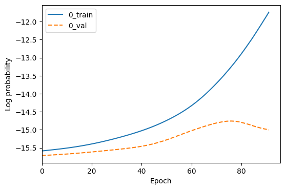
Plotting model loss¶

We can plot the model loss using the fitter.plot_loss method. This method will create a plot of the training and validation loss over epochs, and save it to the plots/ directory in the output folder for this model. By default, it will not overwrite existing plots, but you can change this with the overwrite argument.

[14]:

fitter.plot_loss(overwrite=True);

../_images/sbi_train_basic_sbi_model_31_0.png

Plotting validation metrics¶

Whilst it does happen automatically during training, we can also plot the validation metrics of a trained model using the fitter.plot_diagnostics method. You can provide your own validation set, or by default it will use the test set from the last training run. By default, it will not create existing plots in the plots/ directory, but you can change this with the overwrite argument.

[15]:

fitter.plot_diagnostics();

2025-11-13 20:07:52,012 | synference | INFO     | [  1.77582467  11.90214539   2.40552688   1.45580852 902.70309172
  -2.10306764]

1275it [00:00, 261336.93it/s]
INFO:root:Saving single posterior plot to /opt/hostedtoolcache/Python/3.10.19/x64/lib/python3.10/models/test/plots/test_19_plot_single_posterior.jpg...

2025-11-13 20:08:00,912 | synference | INFO     | shapes: X:(20, 8), y:(20, 6)

100%|██████████| 20/20 [00:00<00:00, 290.88it/s]
INFO:root:Saving posterior samples to /opt/hostedtoolcache/Python/3.10.19/x64/lib/python3.10/models/test/plots/posterior_samples.npy...
INFO:root:Saving coverage plot to /opt/hostedtoolcache/Python/3.10.19/x64/lib/python3.10/models/test/plots/plot_coverage.jpg...
INFO:root:Saving ranks histogram to /opt/hostedtoolcache/Python/3.10.19/x64/lib/python3.10/models/test/plots/ranks_histogram.jpg...
INFO:root:Mean logprob: -1.4686e+01Median logprob: -1.4053e+01
INFO:root:Saving true logprobs to /opt/hostedtoolcache/Python/3.10.19/x64/lib/python3.10/models/test/plots/true_logprobs.npy...
INFO:root:Saving true logprobs plot to /opt/hostedtoolcache/Python/3.10.19/x64/lib/python3.10/models/test/plots/plot_true_logprobs.jpg...
INFO:matplotlib.mathtext:Substituting symbol E from STIXNonUnicode
100%|██████████| 100/100 [00:00<00:00, 708.06it/s]

../_images/sbi_train_basic_sbi_model_33_4.png

../_images/sbi_train_basic_sbi_model_33_5.png

../_images/sbi_train_basic_sbi_model_33_6.png

../_images/sbi_train_basic_sbi_model_33_7.png

INFO:matplotlib.mathtext:Substituting symbol E from STIXNonUnicode

../_images/sbi_train_basic_sbi_model_33_9.png

../_images/sbi_train_basic_sbi_model_33_10.png

Getting model metrics¶

We can print and save metrics of the trained model using the fitter.evaluate_model method. This method will print the metrics to the console, and also save them to a .json file in the output directory for this model. The metrics include:

TARP (Tests of Accuracy with Random Points)
Log DPIT (Logarithmic Deviation of the Probability Integral Transform)
Mean Log Probability
Parameter-specific metrics (MSE, RMSE, Mean Absolute Error, Median Absolute Error, R-squared, Normalized RMSE)

[16]:

fitter.evaluate_model();

Sampling from posterior: 100%|██████████| 20/20 [00:00<00:00, 244.07it/s]
100%|██████████| 200/200 [00:00<00:00, 696.51it/s]
Log prob: 100%|██████████| 20/20 [00:00<00:00, 84.45it/s]

2025-11-13 20:08:05,967 | synference | INFO     | ============================================================
2025-11-13 20:08:05,968 | synference | INFO     | MODEL PERFORMANCE METRICS
2025-11-13 20:08:05,969 | synference | INFO     | ============================================================
2025-11-13 20:08:05,970 | synference | INFO     | Full Model Metrics:
2025-11-13 20:08:05,970 | synference | INFO     | ----------------------------------------
2025-11-13 20:08:05,971 | synference | INFO     | TARP..................... 0.193500
2025-11-13 20:08:05,972 | synference | INFO     | LOG DPIT MAX............. 0.550212
2025-11-13 20:08:05,972 | synference | INFO     | MEAN LOG PROB............ -15.009567
2025-11-13 20:08:05,973 | synference | INFO     | Parameter-Specific Metrics:
2025-11-13 20:08:05,974 | synference | INFO     | ----------------------------------------
2025-11-13 20:08:05,975 | synference | INFO     | Metric        redshift  log_mass     tau_v       tau        peak_age  log10metallicity
2025-11-13 20:08:05,976 | synference | INFO     | --------------------------------------------------------------------------------------
2025-11-13 20:08:05,976 | synference | INFO     | MSE           1.612745  0.662789  0.556009  0.332795  2615607.195786          0.643579
2025-11-13 20:08:05,977 | synference | INFO     | RMSE          1.269939  0.814119  0.745660  0.576884     1617.283895          0.802234
2025-11-13 20:08:05,978 | synference | INFO     | MEAN AE       0.972638  0.711508  0.632357  0.488750     1464.478911          0.699265
2025-11-13 20:08:05,979 | synference | INFO     | MEDIAN AE     0.704399  0.673034  0.608911  0.460172     1429.285011          0.755862
2025-11-13 20:08:05,979 | synference | INFO     | R SQUARED     0.999958  0.999981  0.999986  0.999991       -0.145381          0.999984
2025-11-13 20:08:05,980 | synference | INFO     | RMSE NORM     0.001977  0.001267  0.001161  0.000898        2.517632          0.001249
2025-11-13 20:08:05,981 | synference | INFO     | MEAN AE NORM  0.001514  0.001108  0.000984  0.000761        2.279760          0.001089
2025-11-13 20:08:05,982 | synference | INFO     | ============================================================

Posterior Samples¶

We can sample the posterior for a given observation using the fitter.sample_posterior method. This method takes an observation, or a set of observations, as an argument, and returns samples from the posterior distribution. If no observation is provided, it will draw posterior samples for all observations in the test set.

[17]:

fitter.sample_posterior()

Sampling from posterior: 100%|██████████| 20/20 [00:00<00:00, 295.83it/s]

[17]:

array([[[ 4.43637657e+00,  1.02292881e+01,  1.54729509e+00,
          1.43596637e+00,  3.16060938e+03, -2.21769428e+00],
        [ 1.45867074e+00,  9.89816284e+00,  9.38274860e-01,
          6.45267248e-01,  2.51038477e+03, -1.89690137e+00],
        [ 1.83080673e+00,  9.34383392e+00,  8.85771036e-01,
          3.62305999e-01,  2.05320947e+03, -3.35116196e+00],
        ...,
        [ 3.38039994e+00,  9.34642982e+00,  4.41242725e-01,
          1.47353172e+00,  2.09725052e+02, -3.73615003e+00],
        [ 3.06743693e+00,  9.56037521e+00,  1.45556641e+00,
          1.12459397e+00,  3.36770874e+03, -3.81893730e+00],
        [ 1.24062002e+00,  1.08276043e+01,  1.65632355e+00,
          1.23617506e+00,  5.78415955e+02, -2.89406824e+00]],

       [[ 2.06275344e+00,  1.15559540e+01,  1.87236881e+00,
          6.79997027e-01,  2.89783887e+03, -1.47195280e+00],
        [ 1.37080359e+00,  1.00598679e+01,  2.18736744e+00,
          8.99465859e-01,  2.14573999e+03, -2.36454487e+00],
        [ 2.18008780e+00,  9.00345421e+00,  8.30197334e-01,
          6.73525631e-01,  9.79495544e+02, -2.37996268e+00],
        ...,
        [ 3.95291662e+00,  1.14550877e+01,  8.73087466e-01,
          1.34637403e+00,  1.12226440e+03, -2.46954203e+00],
        [ 3.74584889e+00,  9.52462387e+00,  1.92294526e+00,
          7.63964891e-01,  3.43177588e+03, -2.53173399e+00],
        [ 2.67332649e+00,  8.22163391e+00,  1.56289709e+00,
          1.48882508e+00,  3.12180615e+03, -2.55249691e+00]],

       [[ 2.12075874e-01,  1.12096701e+01,  2.13162017e+00,
          1.77222586e+00,  9.80960156e+03, -2.11917114e+00],
        [ 1.26868905e-02,  1.08154182e+01,  9.15760219e-01,
          1.22273731e+00,  5.03601758e+03, -2.31831980e+00],
        [ 1.83458924e+00,  1.11357527e+01,  8.24464202e-01,
          1.06957972e+00,  1.76367493e+03, -3.75751638e+00],
        ...,
        [ 1.49825621e+00,  1.08259258e+01,  2.59762907e+00,
          1.52266479e+00,  2.90986719e+03, -2.89687443e+00],
        [ 1.34700561e+00,  1.00425177e+01,  1.97565734e+00,
          1.74205410e+00,  3.72194775e+03, -2.32829261e+00],
        [ 2.68690157e+00,  1.09255733e+01,  5.87903380e-01,
          1.45694029e+00,  6.06308154e+03, -3.12207222e+00]],

       ...,

       [[ 2.09123945e+00,  9.72378159e+00,  1.69266534e+00,
          1.11699057e+00,  3.75991272e+02, -2.72509933e+00],
        [ 1.65267393e-01,  1.16307077e+01,  3.59977782e-01,
          2.23727971e-01,  1.14234692e+03, -3.80817533e+00],
        [ 3.63801575e+00,  1.02194862e+01,  2.06423640e+00,
          9.45030630e-01,  3.28833423e+03, -1.83303189e+00],
        ...,
        [ 1.92830873e+00,  1.16306124e+01,  1.38150477e+00,
          1.73853076e+00,  3.12695337e+03, -2.71629190e+00],
        [ 4.33787346e+00,  1.02398720e+01,  1.76743150e+00,
          1.81650341e+00,  1.35504150e+03, -1.68158424e+00],
        [ 1.60695362e+00,  9.45543575e+00,  6.60745502e-01,
          9.91216660e-01,  4.29621777e+03, -2.23841453e+00]],

       [[ 1.88469338e+00,  1.19160366e+01,  8.93945873e-01,
          8.30852389e-01,  1.47671826e+03, -3.78907561e+00],
        [ 2.31543159e+00,  1.12522268e+01,  2.99257934e-01,
          1.44575334e+00,  2.92752563e+03, -3.45438600e+00],
        [ 1.68705434e-01,  9.87287140e+00,  6.42248094e-01,
          7.06860423e-01,  3.13403345e+03, -3.24074149e+00],
        ...,
        [ 5.99716485e-01,  9.17316341e+00,  1.30009484e+00,
          8.57969284e-01,  6.98829736e+03, -3.27258778e+00],
        [ 1.70158029e+00,  1.16666241e+01,  2.04721832e+00,
          1.40421605e+00,  1.93691443e+03, -3.95289898e+00],
        [ 6.10725701e-01,  1.11951561e+01,  2.01352850e-01,
          1.12558007e+00,  3.09887622e+03, -3.12899852e+00]],

       [[ 2.02615476e+00,  9.06091595e+00,  1.13941419e+00,
          1.23710120e+00,  1.21803162e+03, -2.45834684e+00],
        [ 1.30348933e+00,  9.65362930e+00,  1.24300349e+00,
          1.45019448e+00,  4.07321997e+03, -2.60561371e+00],
        [ 8.21598828e-01,  1.11123257e+01,  8.01883101e-01,
          1.17598021e+00,  6.13376807e+03, -3.81909609e+00],
        ...,
        [ 1.33904648e+00,  9.57715321e+00,  3.12093705e-01,
          5.19142568e-01,  7.83852539e+02, -3.72919059e+00],
        [ 1.98047018e+00,  1.09033842e+01,  1.56945258e-01,
          1.80692852e-01,  2.85257471e+03, -3.32650137e+00],
        [ 1.39164507e+00,  1.03526907e+01,  1.39965069e+00,
          1.77379739e+00,  2.16916675e+03, -3.71562672e+00]]],
      shape=(20, 1000, 6))

Next Steps¶

In the next tutorials, we will cover more advanced configurations for training SBI models, including different feature and parameter configurations, different NDEs, and different prior proposals. We will also cover how to use the trained models for inference on real data.