Synthesizer Crash Course
Getting Started
Synthesizer is a Python package designed to create synthetic astronomical observables from both parametric models and hydrodynamical simulations. It is built to be flexible and modular, allowing users to easily customize and extend its functionality.
You should already have Synthesizer installed if you have followed the installation instructions for Synference. If not, you can run:
pip install cosmos-synthesizer
Synthesizer Grids
Synthesizer relies on pre-computed SPS (Stellar Population Synthesis) model grids to generate synthetic observables. The main documentation for these grids can be found here. Pre-computed grids are available for download for several popular SPS models, including: BPASS, FSPS, BC03, and Maraston, and are stored in HDF5 format.
Additionally, pre-computed grids have been generated for a variety of IMFs, and variants which have been post-processed to include nebular emission using Cloudy are also available.
For the purposes of this crash course, we will use a test grid from BPASS v2.2.1, but the following will work with any of the available grids.
Grids are handled using the synthesizer.Grid class, where the grid_dir argument tells the code where the desired Grid lives.
Here is some code to download the grids using the synthesizer-download command.
import subprocess

subprocess.Popen(["synthesizer-download", "--test-grids", "--dust-grid"])`
[1]:
from synthesizer import Grid

grid = Grid("test_grid")
unyt
Synthesizer uses the unyt package to handle physical units. You can find more information about unyt here.
[2]:
from unyt import Kelvin, Msun, Myr
Instruments and Filters
Synthesizer includes a variety of built-in instruments and filters, which can be found in the documentation. You can also add your own custom filters if needed, and any filter from SVO can be used with the OBSERVATORY/INSTRUMENT.FILTER syntax, e.g. JWST/NIRCam.F356W.
Individual filters are stored in the Filter class, and collection of filters are stored in FilterCollection.
An Instrument stores a FilterCollection as well as other information about the instrument, such as its name and the observatory it belongs to.
For this crash course, we will use a premade instrument which contains all the wide filters for JWST NIRCam, which we can plot.
[3]:
from synthesizer.instruments.filters import Filter

filter = Filter("JWST/NIRCam.F356W")

from synthesizer.instruments import JWSTNIRCamWide

nircam = JWSTNIRCamWide()

nircam.filters.plot_transmission_curves()
---------------------------------------------------------------------------
TimeoutError                              Traceback (most recent call last)
File /opt/hostedtoolcache/Python/3.10.20/x64/lib/python3.10/urllib/request.py:1348, in AbstractHTTPHandler.do_open(self, http_class, req, **http_conn_args)
   1347 try:
-> 1348     h.request(req.get_method(), req.selector, req.data, headers,
   1349               encode_chunked=req.has_header('Transfer-encoding'))
   1350 except OSError as err: # timeout error

File /opt/hostedtoolcache/Python/3.10.20/x64/lib/python3.10/http/client.py:1303, in HTTPConnection.request(self, method, url, body, headers, encode_chunked)
   1302 """Send a complete request to the server."""
-> 1303 self._send_request(method, url, body, headers, encode_chunked)

File /opt/hostedtoolcache/Python/3.10.20/x64/lib/python3.10/http/client.py:1349, in HTTPConnection._send_request(self, method, url, body, headers, encode_chunked)
   1348     body = _encode(body, 'body')
-> 1349 self.endheaders(body, encode_chunked=encode_chunked)

File /opt/hostedtoolcache/Python/3.10.20/x64/lib/python3.10/http/client.py:1298, in HTTPConnection.endheaders(self, message_body, encode_chunked)
   1297     raise CannotSendHeader()
-> 1298 self._send_output(message_body, encode_chunked=encode_chunked)

File /opt/hostedtoolcache/Python/3.10.20/x64/lib/python3.10/http/client.py:1058, in HTTPConnection._send_output(self, message_body, encode_chunked)
   1057 del self._buffer[:]
-> 1058 self.send(msg)
   1060 if message_body is not None:
   1061
   1062     # create a consistent interface to message_body

File /opt/hostedtoolcache/Python/3.10.20/x64/lib/python3.10/http/client.py:996, in HTTPConnection.send(self, data)
    995 if self.auto_open:
--> 996     self.connect()
    997 else:

File /opt/hostedtoolcache/Python/3.10.20/x64/lib/python3.10/http/client.py:962, in HTTPConnection.connect(self)
    961 sys.audit("http.client.connect", self, self.host, self.port)
--> 962 self.sock = self._create_connection(
    963     (self.host,self.port), self.timeout, self.source_address)
    964 # Might fail in OSs that don't implement TCP_NODELAY

File /opt/hostedtoolcache/Python/3.10.20/x64/lib/python3.10/socket.py:857, in create_connection(address, timeout, source_address)
    856 try:
--> 857     raise err
    858 finally:
    859     # Break explicitly a reference cycle

File /opt/hostedtoolcache/Python/3.10.20/x64/lib/python3.10/socket.py:845, in create_connection(address, timeout, source_address)
    844     sock.bind(source_address)
--> 845 sock.connect(sa)
    846 # Break explicitly a reference cycle

TimeoutError: [Errno 110] Connection timed out

During handling of the above exception, another exception occurred:

URLError                                  Traceback (most recent call last)
File /opt/hostedtoolcache/Python/3.10.20/x64/lib/python3.10/site-packages/synthesizer/instruments/filters.py:2041, in Filter._make_svo_filter(self)
   2040 try:
-> 2041     with urllib.request.urlopen(self.svo_url) as f:
   2042         # Get the root of the XML tree
   2043         root = ElementTree.parse(f).getroot()

File /opt/hostedtoolcache/Python/3.10.20/x64/lib/python3.10/urllib/request.py:216, in urlopen(url, data, timeout, cafile, capath, cadefault, context)
    215     opener = _opener
--> 216 return opener.open(url, data, timeout)

File /opt/hostedtoolcache/Python/3.10.20/x64/lib/python3.10/urllib/request.py:519, in OpenerDirector.open(self, fullurl, data, timeout)
    518 sys.audit('urllib.Request', req.full_url, req.data, req.headers, req.get_method())
--> 519 response = self._open(req, data)
    521 # post-process response

File /opt/hostedtoolcache/Python/3.10.20/x64/lib/python3.10/urllib/request.py:536, in OpenerDirector._open(self, req, data)
    535 protocol = req.type
--> 536 result = self._call_chain(self.handle_open, protocol, protocol +
    537                           '_open', req)
    538 if result:

File /opt/hostedtoolcache/Python/3.10.20/x64/lib/python3.10/urllib/request.py:496, in OpenerDirector._call_chain(self, chain, kind, meth_name, *args)
    495 func = getattr(handler, meth_name)
--> 496 result = func(*args)
    497 if result is not None:

File /opt/hostedtoolcache/Python/3.10.20/x64/lib/python3.10/urllib/request.py:1377, in HTTPHandler.http_open(self, req)
   1376 def http_open(self, req):
-> 1377     return self.do_open(http.client.HTTPConnection, req)

File /opt/hostedtoolcache/Python/3.10.20/x64/lib/python3.10/urllib/request.py:1351, in AbstractHTTPHandler.do_open(self, http_class, req, **http_conn_args)
   1350 except OSError as err: # timeout error
-> 1351     raise URLError(err)
   1352 r = h.getresponse()

URLError: <urlopen error [Errno 110] Connection timed out>

During handling of the above exception, another exception occurred:

SVOInaccessible                           Traceback (most recent call last)
Cell In[3], line 3
      1 from synthesizer.instruments.filters import Filter
----> 3 filter = Filter("JWST/NIRCam.F356W")
      5 from synthesizer.instruments import JWSTNIRCamWide
      7 nircam = JWSTNIRCamWide()

File /opt/hostedtoolcache/Python/3.10.20/x64/lib/python3.10/site-packages/synthesizer/units.py:909, in accepts.<locals>.check_accepts.<locals>.wrapped(*args, **kwargs)
    906 finally:
    907     toc(f"accepts({func.__qualname__})")
--> 909 return func(*bound.args, **bound.kwargs)

File /opt/hostedtoolcache/Python/3.10.20/x64/lib/python3.10/site-packages/synthesizer/utils/operation_timers.py:98, in timed.<locals>.decorator.<locals>.wrapped(*args, **kwargs)
     94 tic(timer_name)
     95 try:
     96     # Return the wrapped function result unchanged so the decorator
     97     # is transparent aside from its timing side effect.
---> 98     return func(*args, **kwargs)
     99 finally:
    100     # Always stop the timer, even if the wrapped function raises,
    101     # so the timing stack remains balanced.
    102     toc(timer_name)

File /opt/hostedtoolcache/Python/3.10.20/x64/lib/python3.10/site-packages/synthesizer/instruments/filters.py:1770, in Filter.__init__(self, filter_code, transmission, lam_min, lam_max, lam_eff, lam_fwhm, new_lam, hdf)
   1768 # Is this an SVO filter?
   1769 elif "/" in filter_code and "." in filter_code:
-> 1770     self._make_svo_filter()
   1772 # Otherwise we haven't got a valid combination of inputs.
   1773 else:
   1774     raise exceptions.InconsistentArguments(
   1775         "Invalid combination of filter inputs. \n For a generic "
   1776         "filter provide a transmission and wavelength array. "
   (...)
   1781         "wavelength or an effective wavelength and FWHM."
   1782     )

File /opt/hostedtoolcache/Python/3.10.20/x64/lib/python3.10/site-packages/synthesizer/instruments/filters.py:2052, in Filter._make_svo_filter(self)
   2049         data = root.find(".//TABLEDATA")
   2051 except URLError:
-> 2052     raise exceptions.SVOInaccessible(
   2053         (
   2054             f"The SVO Database at {self.svo_url} "
   2055             "is not responding. Is it down?"
   2056         )
   2057     )
   2059 # Throw an error if we didn't find the filter.
   2060 if field is None:

SVOInaccessible: The SVO Database at http://svo2.cab.inta-csic.es/theory/fps/fps.php?ID=JWST/NIRCam.F356W is not responding. Is it down?
Creating a Mock Galaxy
Synthesizer has a framework for creating mock galaxies using parametric and particle models. Here we will focus on the parametric models, but you can find more information about the particle models in the documentation.
The framework for creating mock galaxies is built around the Galaxy class. A Galaxy contains a stellar component, which is a Stars instance. The Stars class uses the SFH and metallicity model, as well as the SPS Grid we created earlier, to generate the stellar population of the galaxy.
[4]:
from synthesizer.parametric import Galaxy, Stars
Before we can create a Stars instance, we need to define a star formation history (SFH) and a metallicity distribution. Let’s start with the SFH.
1. Define Star Formation History
Synthesizer includes several built-in star formation history (SFH) models, including commonly used models such as:
Constant
Exponential
Delayed Exponential
Lognormal
Double Power Law
These parametric models are typically defined by 1-3 parameters, which can be specified when creating the SFH instance. You can also create your own custom SFH models by subclassing the SFH class.
In this example we will use a simple constant SFH, which is defined by two parameters min_age and max_age, which define the age range over which the SFH is constant. We do not define a Star Formation Rate (SFR) or total mass here, as the SFH will be normalized to the total mass we provide when creating the Stars instance.
[5]:
from synthesizer.parametric import SFH

sfh_history = SFH.Constant(min_age=0 * Myr, max_age=100 * Myr)
We can plot the SFH using the plot_sfh method, and see that it is constant between 0 and 100 Myr.
[6]:
sfh_history.plot_sfh(t_range=(0, 2e8))

2. Define Metallicity Distributions
As SPS grids are typically defined over both age and metallicity, we also need to define a metallicity distribution for our stellar population. Synthesizer includes several built-in metallicity distribution models, including:
Delta Function
Gaussian
Here we will use a simple delta function, which is defined by a single parameter metallicity, which defines the metallicity of all stars in the population. The metallicity here is defined as the mass fraction of metals, so a metallicity of 0.02 corresponds (approximately) to solar metallicity.
[7]:
from synthesizer.parametric import ZDist

metal_dist = ZDist.DeltaConstant(metallicity=0.02)
3. Creating the Galaxy
Now that we have defined the SFH and metallicity distribution, we can create a Stars instance. The Stars class takes the age and metallicity arrays of the SPS grid, the SFH and metallicity distribution instances, and the total stellar mass of the population as input.
[8]:
stellar_component = Stars(
    grid.log10ages,
    grid.metallicities,
    sf_hist=sfh_history,
    metal_dist=metal_dist,
    initial_mass=1e10 * Msun,
)
/opt/hostedtoolcache/Python/3.10.20/x64/lib/python3.10/site-packages/unyt/array.py:1900: RuntimeWarning: divide by zero encountered in log10
  out_arr = func(np.asarray(inp), out=out_func, **kwargs)
Now we can finally create a Galaxy instance, which takes the Stars instance as input. The Galaxy class can also take additional components, such as gas or a black hole model, but we will not include those in this example. The Galaxy object also takes a redshift parameter, which is used to calculate the luminosity distance and apply cosmological redshifting to the SED.
[9]:
galaxy = Galaxy(stars=stellar_component, redshift=1)
3. Defining your Emission Model
We now have a Galaxy, but we need to define how to generate the SED from its stellar populations. This is the job of an EmissionModel, which takes the galaxy properties (like stellar masses, ages, and metallicities) and combines them with a pre-computed Grid to produce the synthetic SED.
Emission models follow a tree-like structure to accurately model the various components of a galaxy SED, such as:
Incident (no nebular emission)
Nebular line emission
Nebular continuum
Full nebular emission (lines + continuum)
Intrinsic (nebular + stellar)
When we include modelling of dust attenuation and emission, non-zero escape fractions, and/or AGN emission, the complexity of the emission model increases significantly. Since the possible combinations of models are extensive, Synthesizer provides a comprehensive library of Premade Emission Models which are listed in the documentation.
We encourage you to explore the emission models in the documentation, as they are too numerous to list here. For this example, we will use a TotalEmission model, which is a pre-built model that generates the final combined spectrum, accounting for stellar, nebular, dust attenuation, and thermal dust emission.
For flexibility, our expected emission model components can be set globally on the emission model, or on individual ‘emitters’, such as the Star or Galaxy instances. For example, we can set the escape fraction of ionizing photons to 0.1 for the entire emission model, or we can set it to 0.2 for just the stellar component of the galaxy.
Below we set the escape fraction (\(f_{esc}\)) to 0.1 for the entire emission model, but if we did not set it here, but instead set it on the Galaxy instance, it would override this value.
Before we create our emission model, we need to define our dust attenuation and emission models. Here we use a simple power-law dust attenuation curve, and a single-temperature blackbody for the dust emission. You can find out more information about the wide range of dust models available in the documentation.
Before instantiating our emission model, we first define the components governing the dust physics:
Dust Attenuation: We use a simple power-law dust attenuation curve
Dust Emission: We define the resulting thermal dust emission using a single-temperature blackbody.
[10]:
from synthesizer.emission_models import Blackbody
from synthesizer.emission_models.attenuation import PowerLaw

dust_curve = PowerLaw(slope=-0.7)
dust_emission_model = Blackbody(temperature=30 * Kelvin)
Now we can create our emission model by supplying the dust components, the SPS grid, and specifying a V-band optical depth (\(\tau_{\rm V}\)) to apply to the emission.
[11]:
from synthesizer.emission_models import TotalEmission

emission_model = TotalEmission(
    grid=grid, dust_curve=dust_curve, tau_v=0.3, dust_emission_model=dust_emission_model
)
We can also plot the emission tree to see the components and complexity of our emission model!
[12]:
emission_model.plot_emission_tree()
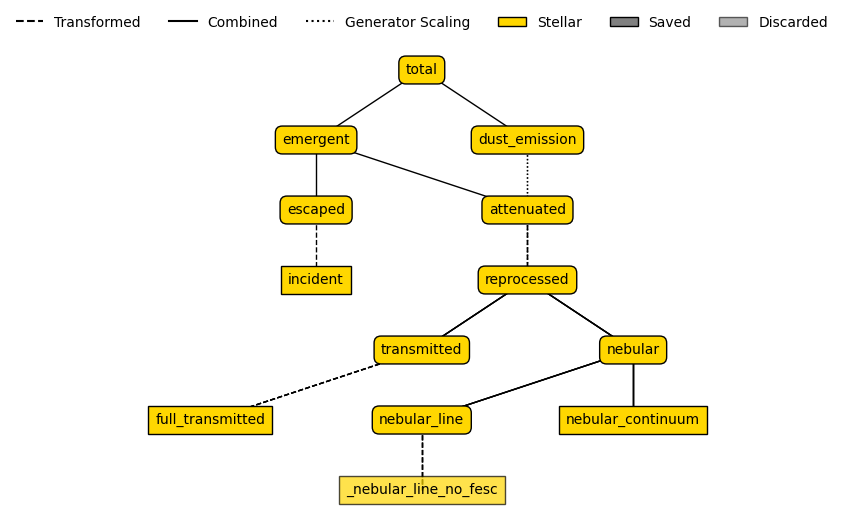
[12]:
(<Figure size 600x600 with 1 Axes>, <Axes: >)
4. Generate observables
Now that we have a galaxy, an emission model, and an instrument, we can generate our synthetic observables. The easiest observable to generate is the galaxy’s rest-frame SED.
This SED is generated by calling the get_spectra method on the Galaxy instance, passing your configured emission model as the argument. This method calculates the complete, integrated SED and returns it as a specialized Sed object, containing the rest-frame wavelength and spectral luminosity density arrays.
Rest-frame SED
[13]:
galaxy.get_spectra(emission_model=emission_model)
galaxy.get_spectra_combined()
/opt/hostedtoolcache/Python/3.10.20/x64/lib/python3.10/site-packages/unyt/array.py:1900: RuntimeWarning: overflow encountered in exp
  out_arr = func(np.asarray(inp), out=out_func, **kwargs)
/opt/hostedtoolcache/Python/3.10.20/x64/lib/python3.10/site-packages/unyt/array.py:2040: RuntimeWarning: overflow encountered in multiply
  out_arr = func(
In addition, the generated spectra for the root emission model and the child models are stored in the galaxy.stars.spectra dictionary. We can plot the total SED, as well as the individual components, such as the stellar and nebular emission by doing the following:
[14]:
galaxy.plot_spectra(stellar_spectra=True)
[14]:
(<Figure size 350x500 with 1 Axes>,
 <Axes: xlabel='$\\lambda/[\\mathrm{\\AA}]$', ylabel='$L_{\\nu}/[\\mathrm{\\rm{erg} \\ / \\ \\rm{Hz \\cdot \\rm{s}}}]$'>)

Observed-frame SED
To convert the rest-frame SED into observed-frame fluxes, you need to define two things: the cosmology and the Intergalactic Medium (IGM) absorption model.
To calculate observed frame fluxes, we need to choose a cosmology. Synthesizer leverages astropy.cosmology for cosmological calculations, allowing you to choose any of the built-in cosmologies (such as the default Plank18), or define your own. For IGM absorption, you must choose a model to account for the attenuation of flux along the line of sight.
Here we will use the default Planck18 cosmology and we choose to use the Inoue2014 IGM model (the only one currently implemented in Synthesizer).
[15]:
from astropy.cosmology import Planck18 as cosmo

galaxy.get_observed_spectra(cosmo=cosmo)
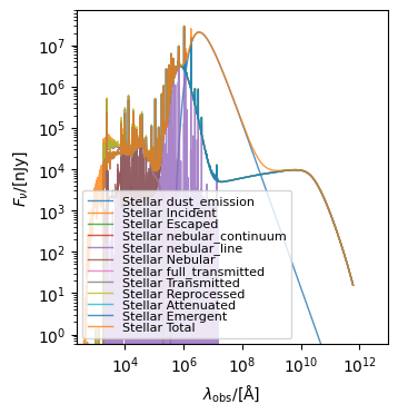
We can plot our observed-frame SED, which includes the effects of cosmological redshifting and IGM absorption:
[16]:
galaxy.plot_observed_spectra(stellar_spectra=True)
[16]:
(<Figure size 350x500 with 1 Axes>,
 <Axes: xlabel='$\\lambda_\\mathrm{obs}/[\\mathrm{\\AA}]$', ylabel='$F_{\\nu}/[\\mathrm{\\rm{nJy}}]$'>)
Photometric Fluxes
To obtain observed photometry through specific bands, we need an Instrument object. This allows our fluxes to be calculated using the get_photo_fnu method, which is available on the Galaxy and Stars objects, and returns a PhotometryCollection object containing the fluxes for every filter specified.
[17]:
fluxes = galaxy.stars.get_photo_fnu(filters=nircam.filters)
---------------------------------------------------------------------------
NameError                                 Traceback (most recent call last)
Cell In[17], line 1
----> 1 fluxes = galaxy.stars.get_photo_fnu(filters=nircam.filters)

NameError: name 'nircam' is not defined
[18]:
print(fluxes["total"])
---------------------------------------------------------------------------
NameError                                 Traceback (most recent call last)
Cell In[18], line 1
----> 1 print(fluxes["total"])

NameError: name 'fluxes' is not defined
Other Calculations
We can calculate other observables, such as emission line fluxes, and equivalent widths, or metadata such as the surviving stellar mass, mass-weighted age or total ionizing luminosity using the appropriate methods of the Galaxy or Stars classes. You can find more information about these methods in the documentation.
Why does this matter?
This core framework, built around grids, galaxy components, and emission models, grants users a high degree of flexibility in generating synthetic observables. By mixing and matching different components, users can construct a vast array of galaxy models tailored to specific astrophysical needs.
This modularity provides the foundation for powerful high-level tools. For instance, the SBI-Fitters library generation tools build directly on this structure to efficiently create the large libraries of synthetic observables needed for simulation-based inference (SBI).
The Synference library generation tools build on this framework to create large libraries of synthetic observables for use in simulation-based inference. You can learn more about library generation in the next section of the documentation.