SED Recovery

In this section, we will discuss the process of recovering the spectral energy distribution (SED) of astronomical sources using the models generated in the previous sections. This will only work if you have a trained inference model, which can be obtained by following the inference tutorial.

For most models created by Synference using Synthesizer, information about the simulator used to generate the model grid is stored in the HDF5 file (e.g. the SPS grid, SFH and metallicity models, emission model, etc). This allows Synference to automatically reconstruct the simulator to generate SEDs for any set of parameters sampled from the posterior distribution.

First we will load in a trained inference model and the corresponding fitter object used to generate the model library.

Note that the manual recreation of the noise model here is only neccessary to get this to work in the documentation. In practice, the noise model should be loaded directly if the path to exists.

You will also need to have the correct model grid (test_grid.hdf5) available in your Synthesizer grid directory for this to work. You can download this from Box.

```python

import os

from synthesizer import get_grids_dir

print(get_grids_dir())

available_grids = os.listdir(get_grids_dir())
if "test_grid.hdf5" not in available_grids:
    cmd = f"synthesizer-download --test-grids --destination {get_grids_dir()}"
    os.system(cmd)

library_path = os.path.join(get_grids_dir(), "test_grid.hdf5")

/home/runner/.local/share/Synthesizer/grids

from synference import SBI_Fitter, load_unc_model_from_hdf5, test_data_dir

library_path = (
    f"{test_data_dir}/grid_BPASS_Chab_DenseBasis_SFH_0.01_z_14_logN_2.7_Calzetti_v3_multinode.hdf5"  # noqa: E501
)

fitter = SBI_Fitter.load_saved_model(
    model_file=f"{test_data_dir}", library_path=library_path, device="cpu"
)

nm_path = f"{test_data_dir}/BPASS_DenseBasis_v4_final_nsf_0_params_empirical_noise_models.h5"
noise_models = load_unc_model_from_hdf5(nm_path)

fitter.feature_array_flags["empirical_noise_models"] = noise_models

/opt/hostedtoolcache/Python/3.10.19/x64/lib/python3.10/site-packages/tqdm/auto.py:21: TqdmWarning: IProgress not found. Please update jupyter and ipywidgets. See https://ipywidgets.readthedocs.io/en/stable/user_install.html
  from .autonotebook import tqdm as notebook_tqdm

2025-11-13 20:02:40,986 | synference | INFO     | Loaded model from /home/runner/.local/share/Synthesizer/data/synference/BPASS_DenseBasis_v4_final_nsf_0_posterior.pkl.
2025-11-13 20:02:40,989 | synference | INFO     | Device: cpu
2025-11-13 20:02:41,082 | synference | WARNING  | IndexError when trying to set train/test arrays.

Now we can recreate the simulator.

fitter.recreate_simulator_from_library(
    override_library_path=library_path, override_grid_path="test_grid.hdf5"
);

2025-11-13 20:02:41,141 | synference | INFO     | Overriding internal library name from provided file path.
2025-11-13 20:02:41,637 | synference | WARNING  | Failed to load cosmology from HDF5. Using Planck18 instead.
2025-11-13 20:02:52,003 | synference | INFO     | Updated filters: ['HST/ACS_WFC.F435W', 'HST/ACS_WFC.F606W', 'HST/ACS_WFC.F775W', 'HST/ACS_WFC.F814W', 'HST/ACS_WFC.F850LP', 'JWST/NIRCam.F090W', 'JWST/NIRCam.F115W', 'JWST/NIRCam.F150W', 'JWST/NIRCam.F200W', 'JWST/NIRCam.F277W', 'JWST/NIRCam.F335M', 'JWST/NIRCam.F356W', 'JWST/NIRCam.F410M', 'JWST/NIRCam.F444W']
2025-11-13 20:02:52,006 | synference | INFO     | Simulator recreated from library at /home/runner/.local/share/Synthesizer/data/synference/grid_BPASS_Chab_DenseBasis_SFH_0.01_z_14_logN_2.7_Calzetti_v3_multinode.hdf5.
2025-11-13 20:02:52,011 | synference | INFO     | Auto applying inverse log10 transform for log10_Av.
2025-11-13 20:02:52,011 | synference | INFO     | Auto applying inverse log10 transform for log10_mass_weighted_age.
2025-11-13 20:02:52,012 | synference | INFO     | Auto applying inverse log10 transform for log10_floor_sfr_10.
2025-11-13 20:02:52,016 | synference | INFO     | Adding Av to tau_v transform.

Now let’s get some mock photometry to recover the SEDs for. We will load a set of mock observations created using the same simulator as the model library.

import numpy as np
from IPython.display import display

path = f"{test_data_dir}/sbi_test_data_BPASS_DenseBasis_v4_final.npz"
data = np.load(path)
X_test = data["X"]
y_test = data["y"]

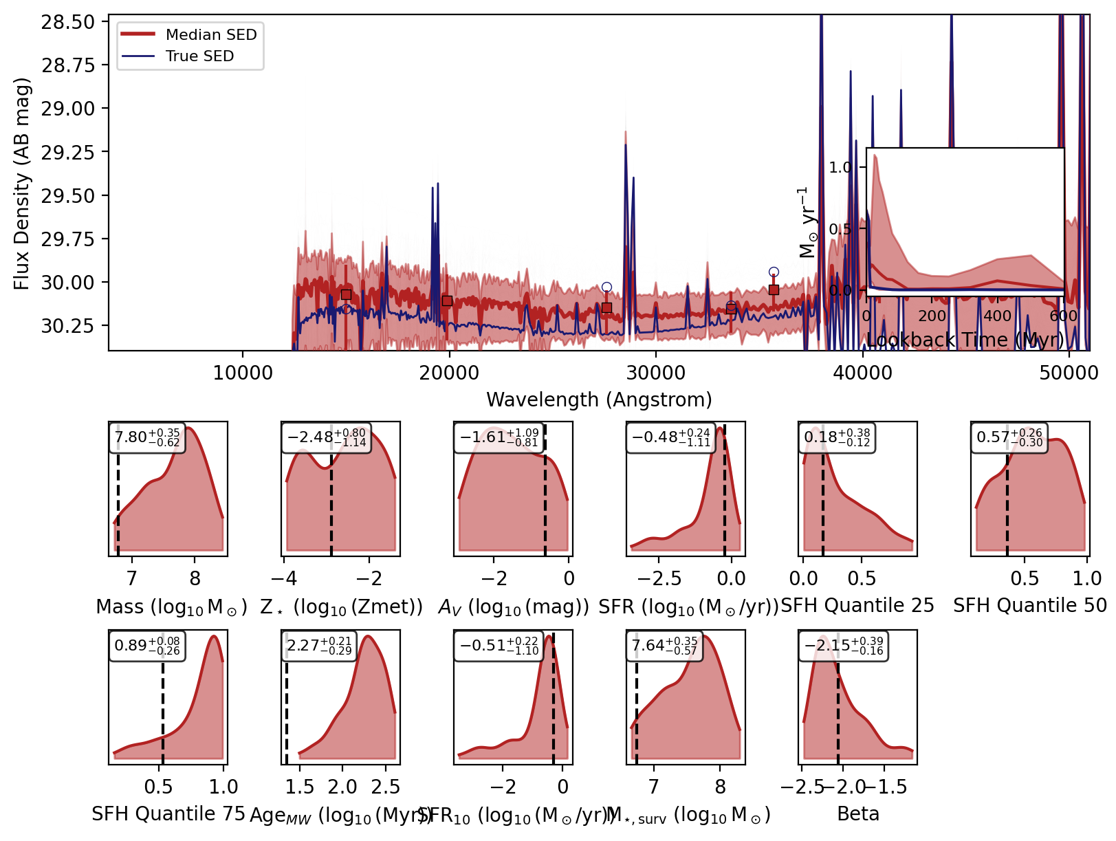
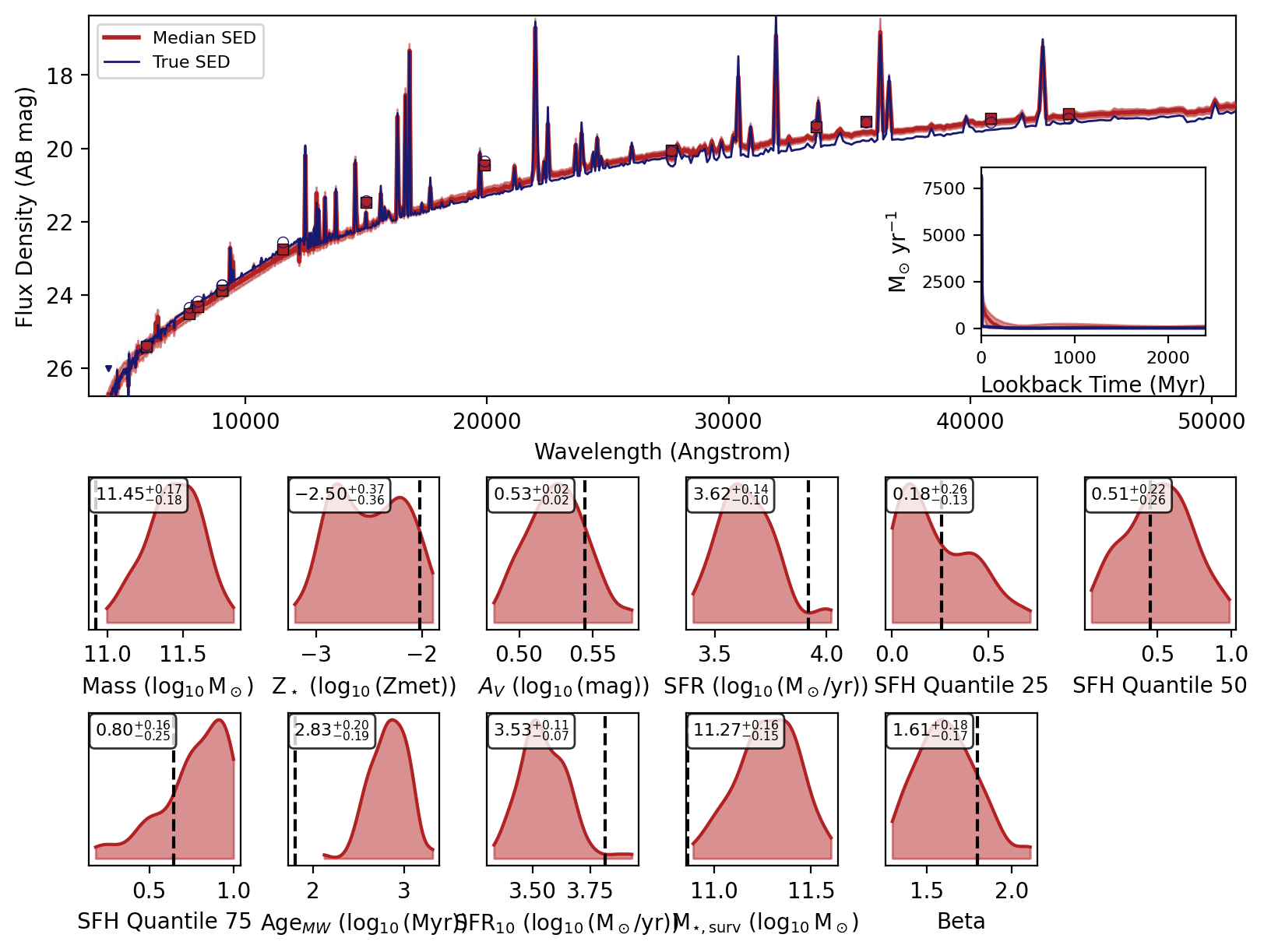
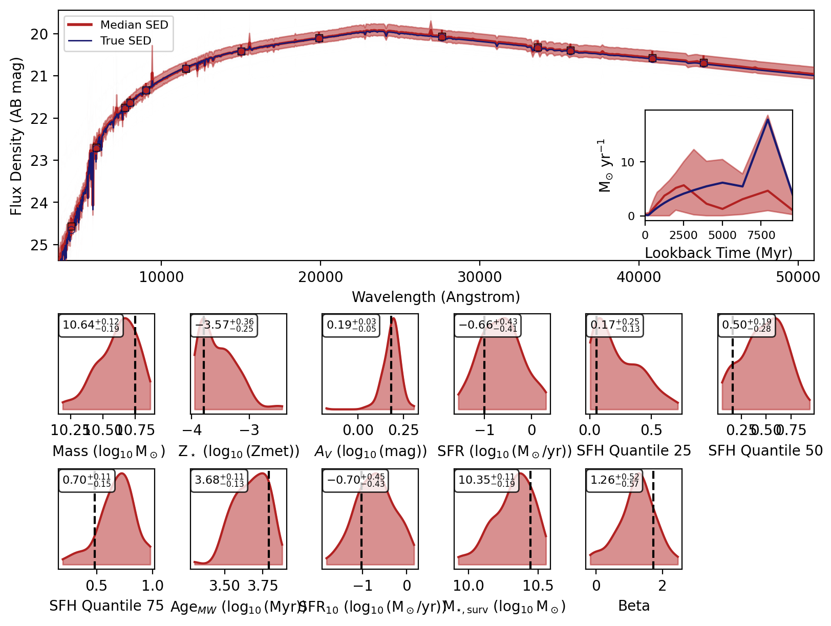
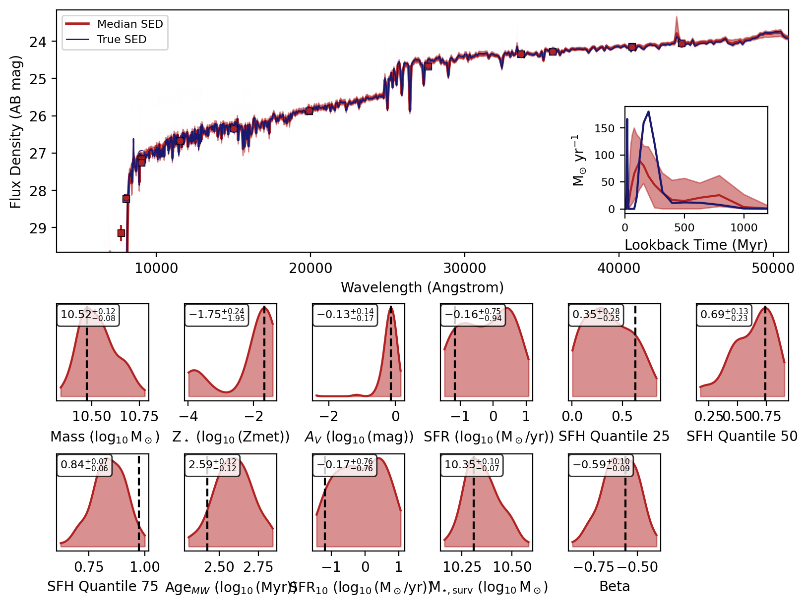
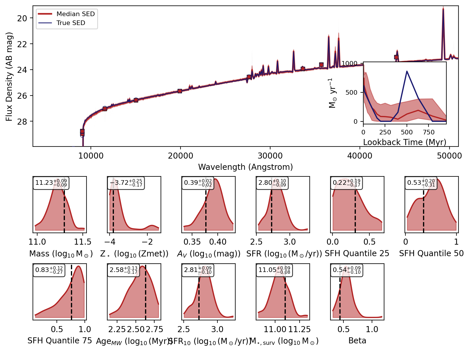
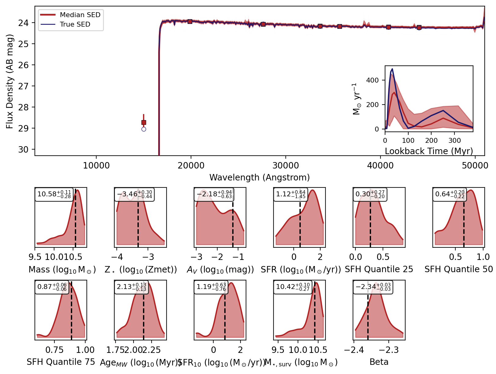
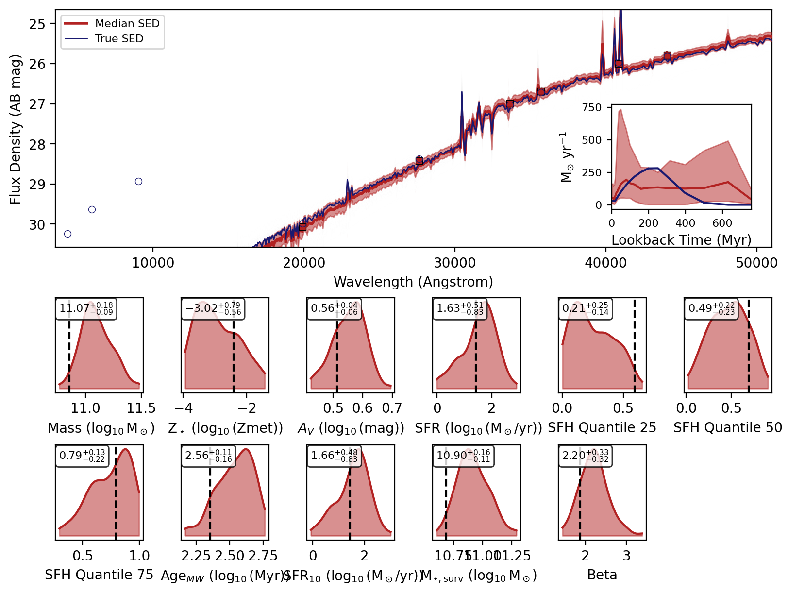
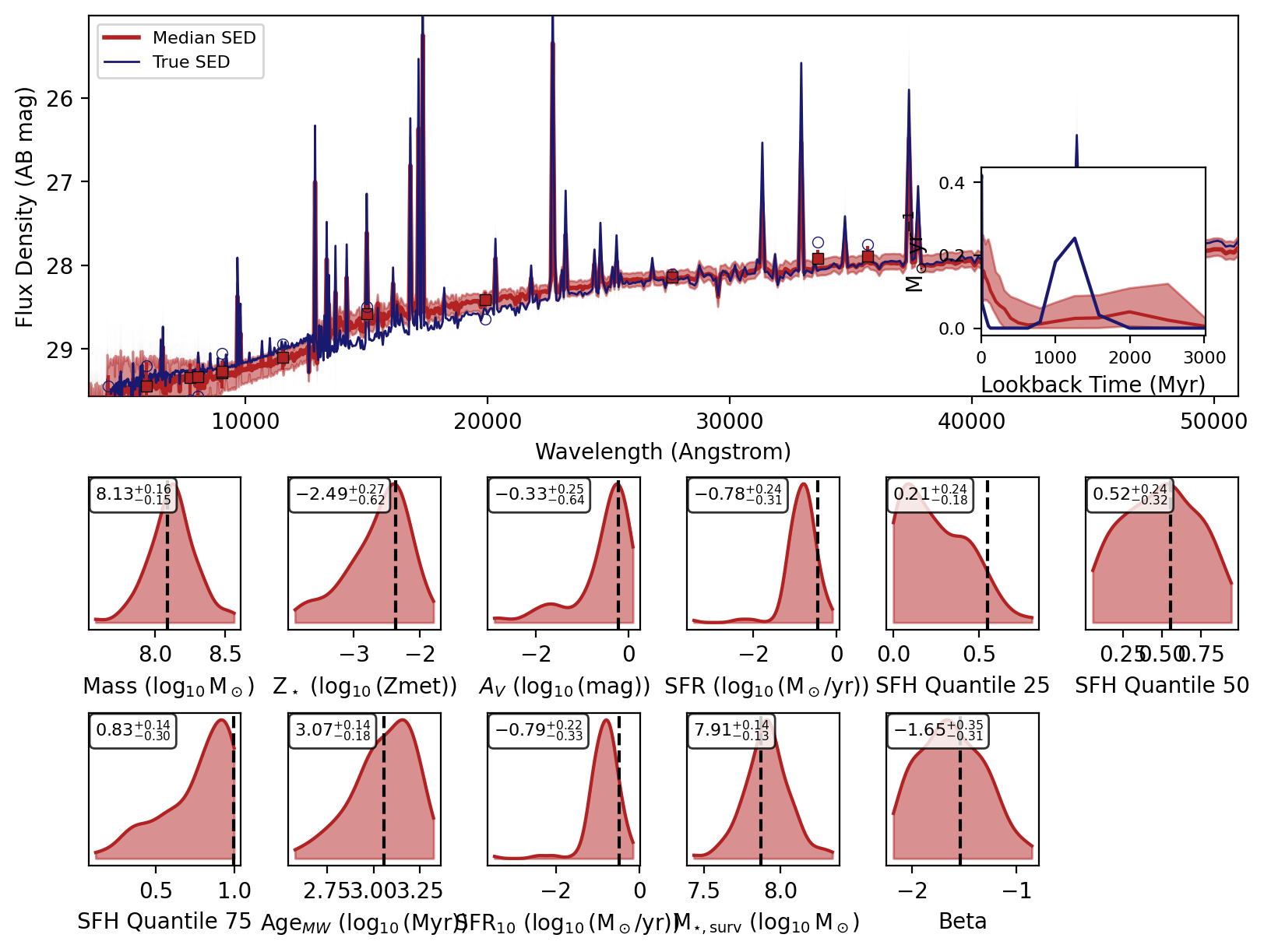
Now we can use the recover_SED method of the inference model to recover the SEDs for our mock photometry. This method will sample from the posterior distribution and generate SEDs for each sample using the reconstructed simulator.

?fitter.recover_SED

Now we will loop over the recovered SEDs and plot them.

%matplotlib inline

for xi_test, yi_test in zip(X_test, y_test):
    _, _, _, _, fig = fitter.recover_SED(
        X_test=xi_test, true_parameters=yi_test, num_samples=100, save_plots=False
    )

    # jupyter notebook display
    display(fig)

Sampling from posterior: 100%|██████████| 1/1 [00:00<00:00,  5.87it/s]
Running simulator on samples:   0%|          | 0/100 [00:00<?, ?it/s]

2025-11-13 20:02:53,220 | synference | WARNING  | The following parameters are not used by the simulator: ['log10_Av', 'log_sfr', 'sfh_quantile_25', 'sfh_quantile_50', 'sfh_quantile_75', 'log10_mass_weighted_age', 'log10_floor_sfr_10', 'log_surviving_mass', 'beta', 'Av', 'mass_weighted_age', 'floor_sfr_10']

Running simulator on samples: 100%|██████████| 100/100 [00:32<00:00,  3.07it/s]

Sampling from posterior: 100%|██████████| 1/1 [00:00<00:00,  8.88it/s]
Running simulator on samples: 100%|██████████| 100/100 [00:38<00:00,  2.58it/s]

Sampling from posterior: 100%|██████████| 1/1 [00:00<00:00,  5.37it/s]
Running simulator on samples: 100%|██████████| 100/100 [00:29<00:00,  3.44it/s]

Sampling from posterior: 100%|██████████| 1/1 [00:00<00:00,  8.11it/s]
Running simulator on samples: 100%|██████████| 100/100 [00:34<00:00,  2.93it/s]

Sampling from posterior: 100%|██████████| 1/1 [00:00<00:00, 11.72it/s]
Running simulator on samples: 100%|██████████| 100/100 [00:27<00:00,  3.59it/s]

Sampling from posterior: 100%|██████████| 1/1 [00:00<00:00, 13.04it/s]
Running simulator on samples: 100%|██████████| 100/100 [00:32<00:00,  3.09it/s]

Sampling from posterior: 100%|██████████| 1/1 [00:00<00:00, 22.40it/s]
Running simulator on samples: 100%|██████████| 100/100 [00:26<00:00,  3.82it/s]

Sampling from posterior: 100%|██████████| 1/1 [00:00<00:00, 17.48it/s]
Running simulator on samples: 100%|██████████| 100/100 [00:17<00:00,  5.56it/s]